Trust Region Policy Optimization

Notes on policy optimization using trust region method.

Preliminaries

Markov Decision Processes

An infinite-horizon discounted Markov Decision Process (MDP) is defined as the tuple $(\mathcal{S},\mathcal{A},P,r,\rho_0,\gamma)$, where

• $\mathcal{S}$ is a finite set of states, or state space.
• $\mathcal{A}$ is a finite set of actions, or action space.
• $P:\mathcal{S}\times\mathcal{A}\times\mathcal{S}\to\mathbb{R}$ is the transition probability distribution, i.e. $P(s,a,s’)=P(s’\vert s,a)$ denotes the probability of transitioning to state $s’$ when taking action $a$ from state $s$.
• $r:\mathcal{S}\times\mathcal{A}\to\mathbb{R}$ is the reward function.
• $\rho_0:\mathcal{S}\to\mathbb{R}$ is the distribution of the initial state $s_0$.
• $\gamma\in(0,1)$ is the discount factor.

A policy, denoted $\pi$, is a mapping from states to probabilities of selecting each possible action, which can be either deterministic $\pi:\mathcal{S}\times\mathcal{A}\to\{0,1\}$ (or $\pi:\mathcal{S}\to\mathcal{A}$) or stochastic $\pi:\mathcal{S}\times\mathcal{A}\to[0,1]$. Here, we consider the stochastic policy only.

We continue by letting $\eta(\pi)$ denoted the expected cumulative discounted reward when starting at initial state $s_0$ and following $\pi$ thereafter \begin{equation} \eta(\pi)=\mathbb{E}_{s_0,a_0,\ldots}\left[\sum_{t=0}^{\infty}\gamma^t r(s_t,a_t)\right], \end{equation} where \begin{equation} s_0\sim\rho_0(s_0),\hspace{1cm}a_t\sim\pi(a_t\vert s_t),\hspace{1cm}s_{t+1}\sim P(s_{t+1}\vert s_t,a_t) \end{equation} For a policy $\pi$, the state value function, denoted as $V_\pi$, of a state $s\in\mathcal{S}$ measures how good it is for the agent to be in $s$, and the action value function, referred as $Q_\pi$, of a state-action pair $(s,a)\in\mathcal{S}\times\mathcal{A}$ specifies how good it is to take action $a$ at state $s$. Specifically, these values are defined by the expected return, as \begin{align} V_\pi(s_t)&=\mathbb{E}_{a_t,s_{t+1},\ldots}\left[\sum_{k=0}^{\infty}\gamma^k r(s_{t+k},a_{t+k})\right], \\ Q_\pi(s_t,a_t)&=\mathbb{E}_{s_{t+1},a_{t+1},\ldots}\left[\sum_{k=0}^{\infty}\gamma^k r(s_{t+k},a_{t+k})\right], \end{align} where \begin{equation} a_t\sim\pi(a_t\vert s_t),\hspace{1cm}s_{t+1}\sim P(s_{t+1}\vert s_t,a_t)\hspace{1cm}t\geq 0 \end{equation} Along with these value functions, we will also define the advantage function for $\pi$, denoted $A_\pi$, given as \begin{equation} A_\pi(s_t,a_t)=Q_\pi(s_t,a_t)-V_\pi(s_t) \end{equation}

Coupling & Total variation distance

Consider two probability measures $\mu$ and $\nu$ on a probability space $(\Omega,\mathcal{F},P)$. One refers a coupling of $\mu$ and $\nu$ as a pair of random variables $(X,Y)$ such that the marginal distribution of $X$ and $Y$ are respectively $\mu$ and $\nu$.

Specifically, if $p$ is a joint distribution of $X,Y$ on $\Omega$, then it implies that \begin{align} \sum_{y\in\Omega}p(x,y)&=\sum_{y\in\Omega}P(X=x,Y=y)=P(X=x)=\mu(x) \\ \sum_{x\in\Omega}p(x,y)&=\sum_{x\in\Omega}P(X=x,Y=y)=P(Y=y)=\nu(y) \end{align} For probability distributions $\mu$ and $\nu$ on $\Omega$ as above, the total variation distance between $\mu$ and $\nu$, denoted $\big\Vert\mu-\nu\big\Vert_\text{TV}$, is defined by \begin{equation} \big\Vert\mu-\nu\big\Vert_\text{TV}\doteq\sup_{A\subset\Omega}\big\vert\mu(A)-\nu(A)\big\vert \end{equation} Proposition 1
Let $\mu$ and $\nu$ be probability distributions on $\Omega$, we then have \begin{equation} \big\Vert\mu-\nu\big\Vert_\text{TV}=\frac{1}{2}\sum_{x\in\Omega}\big\vert\mu(x)-\nu(x)\big\vert \end{equation} Proof
Let $B=\{x:\mu(x)\geq\nu(x)\}$ and let $A\subset\Omega$. We have \begin{align} \mu(A)-\nu(A)&=\mu(A\cap B)+\mu(A\cap B^c)-\nu(A\cap B)-\nu(A\cap B^c) \\ &\leq\mu(A\cap B)-\nu(A\cap B) \\ &\leq\mu(B)-\nu(B) \end{align} Analogously, we also have \begin{equation} \nu(A)-\mu(A)\leq\nu(B^c)-\mu(B^c) \end{equation} Hence, combining these results gives us \begin{equation} \big\Vert\mu-\nu\big\Vert_\text{TV}=\frac{1}{2}\left(\mu(B)-\nu(B)+\nu(B^c)-\mu(B^c)\right)=\frac{1}{2}\sum_{x\in\Omega}\big\vert\mu(x)-\nu(x)\big\vert \end{equation} This proof also implies that \begin{equation} \big\Vert\mu-\nu\big\Vert_\text{TV}=\sum_{x\in\Omega;,\mu(x)\geq\nu(x)}\mu(x)-\nu(x) \end{equation} Proposition 2
Let $\mu$ and $\nu$ be two probability measures defined in a probability space $\Omega$, we then have that \begin{equation} \big\Vert\mu-\nu\big\Vert_\text{TV}=\inf_{(X,Y)\text{ coupling of }\mu,\nu}P(X\neq Y) \end{equation} Proof
For any $A\subset\Omega$ and for any coupling $(X,Y)$ of $\mu$ and $\nu$ we have \begin{align} \mu(A)-\nu(A)&=P(X\in A)-P(Y\in A) \\ &=P(X\in A,Y\notin A)+P(X\in A,Y\in A)-P(Y\in A) \\ &\leq P(X\in A,Y\notin A) \\ &\leq P(X\neq Y), \end{align} which implies that \begin{equation} \big\Vert\mu-\nu\big\Vert_\text{TV}=\sup_{A’\subset\Omega}\big\vert\mu(A’)-\nu(A’)\big\vert\leq P(X\neq Y)\leq\inf_{(X,Y)\text{ coupling of }\mu,\nu}P(X\neq Y) \end{equation} Thus, it suffices to construct a coupling $(X,Y)$ of $\mu$ and $\nu$ such that \begin{equation} \big\Vert\mu-\nu\big\Vert_\text{TV}=P(X\neq Y) \end{equation}

Policy improvement

We begin by proving an identity that expresses the expected return $\eta(\tilde{\pi})$ of a policy $\tilde{\pi}$ in terms of the advantage over another policy $\pi$, accumulated over time steps.

Lemma 3
Given two policies $\pi,\tilde{\pi}$, we have \begin{equation} \eta(\tilde{\pi})=\eta(\pi)+\mathbb{E}_{\tilde{\pi}}\left[\sum_{t=0}^{\infty}\gamma^t A_\pi(s_t,a_t)\right]\label{eq:pi.1} \end{equation} Proof
By definition of advantage function $A_\pi$ of policy $\pi$, we have \begin{align} \mathbb{E}_{\tilde{\pi}}\left[\sum_{t=0}^{\infty}\gamma^t A_\pi(s_t,a_t)\right]&=\mathbb{E}_{\tilde{\pi}}\left[\sum_{t=0}^{\infty}\gamma^t\left(Q_\pi(s_t,a_t)-V_\pi(s_t)\right)\right] \\ &=\mathbb{E}_{\tilde{\pi}}\left[\sum_{t=0}^{\infty}\gamma^t\big(r(s_t,a_t)+\gamma V_\pi(s_{t+1})-V_\pi(s_t)\big)\right] \\ &=\mathbb{E}_{\tilde{\pi}}\left[-V_\pi(s_0)+\sum_{t=0}^{\infty}\gamma^t r(s_t,a_t)\right] \\ &=-\mathbb{E}_{s_0}\big[V_\pi(s_0)\big]+\mathbb{E}_{\tilde{\pi}}\left[\sum_{t=0}^{\infty}\gamma^t r(s_t,a_t)\right] \\ &=-\eta(\pi)+\eta(\tilde{\pi}), \end{align} where in the third step, since $\gamma\in(0,1)$ as $t\to\infty$, we have that $\gamma^t V_\pi(s_{t+1})\to 0$.

Let $\rho_\pi$ be the unnormalized discounted visitation frequencies for state $s$: \begin{equation} \rho_\pi(s)\doteq P(s_0=s)+\gamma P(s_1=s)+\gamma^2 P(s_2=s)+\ldots \end{equation} where $s_0\sim\rho_0$ and the actions are chosen according to $\pi$. This allows us to rewrite \eqref{eq:pi.1} as \begin{align} \eta(\tilde{\pi})&=\eta(\pi)+\sum_{t=0}^{\infty}\sum_{s}P(s_t=s\vert\tilde{\pi})\sum_{a}\tilde{\pi}(a\vert s)\gamma^t A_\pi(s,a) \\ &=\eta(\pi)+\sum_{s}\sum_{t=0}^{\infty}\gamma^t P(s_t=s\vert\tilde{\pi})\sum_{a}\tilde{\pi}(a\vert s)A_\pi(s,a) \\ &=\eta(\pi)+\sum_{s}\rho_\tilde{\pi}(s)\sum_{a}\tilde{\pi}(a\vert s)A_\pi(s,a)\label{eq:pi.2} \end{align} This result implies that any policy update $\pi\to\tilde{\pi}$ that has a nonnegative expected advantage at every state $s$, i.e. $\sum_{a}\tilde{\pi}(a\vert s)A_\pi(s,a)\geq 0$, is guaranteed to make an improvement on $\eta$ (or unchanged in case the expected advantage take the value of zero for every $s$). By letting $\tilde{\pi}$ be the deterministic policy that \begin{equation} \tilde{\pi}(s)=\underset{a}{\text{argmax}}\hspace{0.1cm}A_\pi(s,a), \end{equation} we obtain the policy improvement result used in policy iteration.

However, there are cases when \eqref{eq:pi.2} is difficult to be optimized, especially when the expected advantage is negative, i.e. $\sum_a\tilde{\pi}(a\vert s)A_\pi(s,a)$, due to estimation and approximation error in the approximate setting. We instead consider a local approximation to $\eta$: \begin{equation} L_\pi(\tilde{\pi})=\eta(\pi)+\sum_s\rho_\pi(s)\sum_a\tilde{\pi}(a\vert s)A_\pi(s,a)\label{eq:pi.5} \end{equation}

If $\pi$ is a policy parameterized by $\theta$, in which $\pi_\theta(a\vert s)$ s differentiable w.r.t $\theta$, we then have for any parameter value $\theta_0$ \begin{align} L_{\pi_{\theta_0}}(\pi_{\theta_0})&=\eta(\pi_{\theta_0}) \\ \nabla_\theta L_{\pi_{\theta_0}}(\pi_\theta)\big\vert_{\theta=\theta_0}&=\nabla_\theta\eta(\pi_\theta)\big\vert_{\theta=\theta_0},\label{eq:pi.6} \end{align} which suggests that a sufficiently small step $\pi_{\theta_0}\to\tilde{\pi}$ that leads to an improvement on $L_{\pi_{\theta_\text{old}}}$ will also make an improvement on $\eta$.

To measure the improvement on updating $\pi_\text{old}\to\pi_\text{new}$, we choose the total variance distance metric, as defined above with an observation that each policy $\pi:\mathcal{S}\times\mathcal{A}\to[0,1]$ can be viewed as a distribution function defined on $\mathcal{S}\times\mathcal{A}$. Thus, those results and definitions mentioned above for probability measures $\mu$ and $\nu$ defined on $\Omega$ can also be applied to policies $\pi$ and $\tilde{\pi}$ specified on $\mathcal{S}\times\mathcal{A}$.

In addition, we need to define some notations:

• Let \begin{equation} \big\Vert\pi-\tilde{\pi}\big\Vert_{\text{TV}}^{\text{max}}\doteq\max_s\big\Vert\pi(\cdot\vert s)-\tilde{\pi}(\cdot\vert s)\big\Vert_\text{TV} \end{equation}
• A policy pair $(\pi,\tilde{\pi})$ is referred as $\alpha$-coupled if it defines a joint distribution $(a,\tilde{a})\vert s$ such that \begin{equation} P(a\neq\tilde{a}\vert s)\leq\alpha,\hspace{1cm}\forall s \end{equation} $\pi$ and $\tilde{\pi}$ will respectively denote the marginal distributions of $a$ and $\tilde{a}$.
  
  Proposition 4
  Let $(\pi,\tilde{\pi})$ be $\alpha$-coupled policy pair, for all $s$, we have \begin{equation} \big\vert\bar{A}(s)\big\vert\leq 2\alpha\max_{s,\tilde{a}}\big\vert A_\pi(s,\tilde{a})\big\vert, \end{equation} where $\bar{A}(s)$ is the expected advantage of $\tilde{\pi}$ over $\pi$ at state $s$, given as \begin{equation} \bar{A}(s)=\mathbb{E}_{\tilde{a}\sim\tilde{\pi}}\big[A_\pi(s,\tilde{a})\big] \end{equation} Proof
  By definition of the advantage function, it is easily noticed that $\mathbb{E}_{a\sim\pi}\big[A_\pi(s,a)\big]=0$, which lets us obtain \begin{align} \bar{A}(s)&=\mathbb{E}_{\tilde{a}\sim\tilde{\pi}}\big[A_\pi(s,\tilde{a})\big] \\ &=\mathbb{E}_{a\sim\pi,\tilde{a}\sim\tilde{\pi}}\big[A_\pi(s,\tilde{a})-A_\pi(s,a)\big] \\ &=P(a\neq\tilde{a}\vert s)\mathbb{E}_{a\sim\pi,\tilde{a}\sim\tilde{\pi}\vert a\neq\tilde{a}}\big[A_\pi(s,\tilde{a})-A_\pi(s,a)\big], \end{align} which by definition of $\alpha$-coupling implies that \begin{equation} \big\vert\bar{A}(s)\big\vert\leq\alpha\cdot 2\max_{s,\tilde{a}}\big\vert A_\pi(s,\tilde{a})\big\vert \end{equation}

Theorem 5
Let $\alpha=\big\Vert\pi-\tilde{\pi}\big\Vert_\text{TV}^\text{max}$. The following holds \begin{equation} \eta(\tilde{\pi})\geq L_\pi(\tilde{\pi})-\frac{4\epsilon\gamma}{(1-\gamma)^2}\alpha^2, \end{equation} where \begin{equation} \epsilon=\max_{s,a}\big\vert A_\pi(s,a)\big\vert \end{equation} Proof

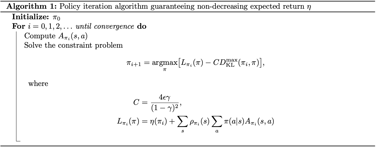
On the other hand, by Pinsker’s inequality, which bounds the total variation distance in terms of the Kullback-Leibler divergence, denoted $D_\text{KL}$, we have that \begin{equation} \big\Vert\pi-\tilde{\pi}\big\Vert_\text{TV}^2\leq\frac{1}{2}D_\text{KL}(\pi\Vert\tilde{\pi})\leq D_\text{KL}(\pi\Vert\tilde{\pi}),\label{eq:pi.3} \end{equation} since $D_\text{KL}(\cdot\Vert\cdot)\geq 0$. Thus, let \begin{equation} D_\text{KL}^\text{max}(\pi,\tilde{\pi})\doteq\max_s D_\text{KL}\big(\pi(\cdot\vert s)\Vert\tilde{\pi}(\cdot\vert s)\big), \end{equation} with the result \eqref{eq:pi.3} and by Theorem 5, we have \begin{equation} \eta(\tilde{\pi})\geq L_\pi(\tilde{\pi})-CD_\text{KL}^\text{max}(\pi,\tilde{\pi}),\label{eq:pi.4} \end{equation} where \begin{equation} C=\frac{4\epsilon\gamma}{(1-\gamma)^2} \end{equation} The policy improvement bound \eqref{eq:pi.4} allows us to specify a policy iteration, as given in the following pseudocode

It is worth noticing that \eqref{eq:pi.4} allows the policy iteration above to guarantee to generating a sequence of non-decreasing expected returns \begin{equation} \eta(\pi_0)\leq\eta(\pi_1)\leq\eta(\pi_2)\leq\ldots \end{equation} To see this, let \begin{equation} M_i(\pi)\doteq L_{\pi_i}(\pi)-CD_\text{KL}^\text{max}(\pi_i,\pi), \end{equation} by \eqref{eq:pi.4}, we then have \begin{equation} \eta(\pi_{i+1})\geq M_i(\pi_{i+1}), \end{equation} which implies that \begin{equation} \eta(\pi_{i+1})-\eta(\pi_i)=\eta(\pi_{i+1})-M_i(\pi_i)\geq M_i(\pi_{i+1})-M_i(\pi_i) \end{equation}

Parameterized Policy Optimization by Trust Region

We now consider the policy optimization problem in which the policy is parameterized by $\theta$.

We begin by simplifying notations. In particular, let $\eta(\theta)\doteq\eta(\pi_\theta)$, let $L_\theta(\tilde{\theta})\doteq L_{\pi_\theta}(\pi_\tilde{\theta})$ and $D_\text{KL}(\theta\Vert\tilde{\theta})\doteq D_\text{KL}(\pi_\theta\Vert\pi_\tilde{\theta})$, which allows us to represent \begin{equation} D_\text{KL}^\text{max}(\theta,\tilde{\theta})\doteq D_\text{KL}^\text{max}(\pi_\theta,\pi_\tilde{\theta})=\max_s D_\text{KL}\big(\pi_\theta(\cdot\vert s)\Vert\pi_\tilde{\theta}(\cdot\vert s)\big) \end{equation} Also let $\theta_\text{old}$ denote the previous policy parameters that we want to improve. Hence, by the previous section, we have \begin{equation} \eta(\theta)\geq L_{\theta_\text{old}}(\theta)-CD_\text{KL}^\text{max}(\theta_\text{old},\theta), \end{equation} where the equality holds at $\theta=\theta_\text{old}$. This means, we get a guaranteed improvement to the true objective function $\eta$ by solving the following optimization problem \begin{equation} \underset{\theta}{\text{maximize}}\hspace{0.2cm}\big[L_{\theta_\text{old}}(\theta)-CD_\text{KL}^\text{max}(\theta_\text{old},\theta)\big] \end{equation} To speed up the algorithm, we make some robust modification. Specifically, we instead solve a trust region problem: \begin{align} \underset{\theta}{\text{maximize}}&\hspace{0.2cm}L_{\theta_\text{old}}(\theta)\nonumber \\ \text{s.t.}&\hspace{0.2cm}\overline{D}_\text{KL}^{\rho_{\theta_\text{old}}}(\theta_\text{old},\theta)\leq\delta,\label{eq:ppo.1} \end{align} where $\overline{D}_\text{KL}^{\rho_{\theta_\text{old}}}$ is the average KL divergence, given as \begin{equation} \overline{D}_\text{KL}^{\rho_{\theta_\text{old}}}(\theta_\text{old},\theta)\doteq\mathbb{E}_{s\sim\rho_{\theta_\text{old}}}\Big[D_\text{KL}\big(\pi_{\theta_\text{old}}(\cdot\vert s)\Vert\pi_\theta(\cdot\vert s)\big)\Big] \end{equation} Let us pay attention to our objective function, $L_{\theta_\text{old}}(\theta)$, for a while. By the definition of $L$, given in \eqref{eq:pi.5}, combined with using an importance sampling estimator, we can rewrite the objective function of \eqref{eq:ppo.1} as \begin{align} L_{\theta_\text{old}}(\theta)&=\sum_s\rho_{\theta_\text{old}}(s)\sum_a\pi_\theta(a\vert s)A_{\theta_\text{old}}(s,a) \\ &=\sum_s\rho_{\theta_\text{old}}(s)\mathbb{E}_{a\sim q}\left[\frac{\pi_\theta(a\vert s)}{q(a\vert s)}A_{\theta_\text{old}}(s,a)\right] \end{align} where $A_{\theta_\text{old}}\doteq A_{\pi_{\theta_\text{old}}}$; and $q$ represents the sampling distribution. The trust region problem now is given as \begin{align} \underset{\theta}{\text{maximize}}&\hspace{0.2cm}\sum_s\rho_{\theta_\text{old}}(s)\mathbb{E}_{a\sim q}\left[\frac{\pi_\theta(a\vert s)}{q(a\vert s)}A_{\theta_\text{old}}(s,a)\right]\nonumber \\ \text{s.t.}&\hspace{0.2cm}\mathbb{E}_{s\sim\rho_{\theta_\text{old}}}\Big[D_\text{KL}\big(\pi_{\theta_\text{old}}(\cdot\vert s)\Vert\pi_\theta(\cdot\vert s)\big)\Big]\leq\delta \end{align} which is thus equivalent to¹² \begin{align} \underset{\theta}{\text{maximize}}&\hspace{0.2cm}\mathbb{E}_{s\sim\rho_{\theta_\text{old}},a\sim q}\left[\frac{\pi_\theta(a\vert s)}{q(a\vert s)}A_{\theta_\text{old}}(s,a)\right]\nonumber \\ \text{s.t.}&\hspace{0.2cm}\mathbb{E}_{s\sim\rho_{\theta_\text{old}}}\Big[D_\text{KL}\big(\pi_{\theta_\text{old}}(\cdot\vert s)\Vert\pi_\theta(\cdot\vert s)\big)\Big]\leq\delta\label{eq:ppo.2} \end{align}

Solving the optimization problem

Let us take a closer look on how to solve this trust region constrained optimization problem. We begin by letting \begin{equation} \mathcal{L}_{\theta_\text{old}}(\theta)\doteq\mathbb{E}_{s\sim\rho_{\theta_\text{old}},a\sim\pi_{\theta_\text{old}}}\left[\frac{\pi_\theta(a\vert s)}{\pi_{\theta_\text{old}}(a\vert s)}A_{\theta_\text{old}}(s,a)\right] \end{equation} Consider Taylor expansion of the objective function $\mathcal{L}_{\theta_\text{old}}(\theta)$ about $\theta=\theta_\text{old}$ to the first order, we thus can linearly approximate the objective function by the policy gradient, $\nabla_\theta\eta(\pi_{\theta_\text{old}})$, as \begin{align} \mathcal{L}_{\theta_\text{old}}(\theta)&\approx\mathbb{E}_{s\sim\rho_{\theta_\text{old}},a\sim\pi_{\theta_\text{old}}}\big[A_{\theta_\text{old}}(s,a)\big]+(\theta-\theta_\text{old})^\text{T}\nabla_\theta\mathcal{L}_{\theta_\text{old}}(\theta)\big\vert_{\theta=\theta_\text{old}} \\ &\overset{\text{(i)}}{=}(\theta-\theta_\text{old})^\text{T}\nabla_\theta\mathcal{L}_{\theta_\text{old}}(\theta)\big\vert_{\theta=\theta_\text{old}} \\ &\overset{\text{(ii)}}{=}(\theta-\theta_\text{old})^\text{T}\left[\frac{1}{1-\gamma}\nabla_\theta L_{\theta_\text{old}}(\theta)\big\vert_{\theta=\theta_\text{old}}\right] \\ &\overset{\text{(iii)}}{=}\frac{1}{1-\gamma}(\theta-\theta_\text{old})^\text{T}\nabla_\theta\eta(\pi_{\theta_\text{old}})\big\vert_{\theta=\theta_\text{old}} \\ &\underset{\max_\theta}{\propto}(\theta-\theta_\text{old})^\text{T}\nabla_\theta\eta(\pi_{\theta_\text{old}})\big\vert_{\theta=\theta_\text{old}},\label{eq:st.1} \end{align} where

• This step is due to definition of advantage function for a policy $\pi$, we have that $\mathbb{E}_{a\sim\pi}\big[A_\pi(s,a)\big]=0$, which implies that \begin{align} \mathbb{E}_{s\sim\rho_{\theta_\text{old}},a\sim\pi_{\theta_\text{old}}}\big[A_{\theta_\text{old}}(s,a)\big]&=\mathbb{E}_{s\sim\rho_{\theta_\text{old}}}\Big[\mathbb{E}_{a\sim\pi_{\theta_\text{old}}}\big[A_{\theta_\text{old}}(s,a)\big]\Big] \\ &=\mathbb{E}_{s\sim\rho_{\theta_\text{old}}}\big[0\big]=0 \end{align}
• This step uses the same logic as we have used in \eqref{eq:fn.1}.
• This step is due to \eqref{eq:pi.6}.

To get an approximation of the constraint, we fist consider the Taylor expansion of the KL divergence $D_\text{KL}\big(\pi_{\theta_\text{old}}(\cdot\vert s)\Vert\pi_\theta(\cdot\vert s)\big)$ about $\theta=\theta_\text{old}$ to the second order, which, given a state $s$, gives us a quadratic approximation: \begin{align} &\hspace{-0.7cm}D_\text{KL}\big(\pi_{\theta_\text{old}}(\cdot\vert s)\Vert\pi_\theta(\cdot\vert s)\big)\nonumber \\ &=\mathbb{E}_{\pi_{\theta_\text{old}}}\Big[\log\pi_{\theta_\text{old}}(\cdot\vert s)-\log\pi_\theta(\cdot\vert s)\Big] \\ &\approx\mathbb{E}_{\pi_{\theta_\text{old}}}\Bigg[\log\pi_{\theta_\text{old}}(\cdot\vert s)-\Big(\log\pi_{\theta_\text{old}}(\cdot\vert s)+(\theta-\theta_\text{old})^\text{T}\nabla_\theta\log\pi_\theta(\cdot\vert s)\big\vert_{\theta=\theta_\text{old}}\nonumber \\ &\hspace{2cm}+\left.\frac{1}{2}(\theta_\text{old}-\theta)^\text{T}\nabla_\theta^2\log\pi_\theta(\cdot\vert s)\big\vert_{\theta=\theta_\text{old}}(\theta_\text{old}-\theta)\right)\Bigg] \\ &\overset{\text{(i)}}{=}-\mathbb{E}_{\pi_{\theta_\text{old}}}\left[\frac{1}{2}(\theta-\theta_\text{old})^\text{T}\nabla_\theta^2\log\pi_\theta(\cdot\vert s)\big\vert_{\theta=\theta_\text{old}}(\theta-\theta_\text{old})\right] \\ &\overset{\text{(ii)}}{=}\frac{1}{2}(\theta-\theta_\text{old})^\text{T}\mathbb{E}_{\pi_{\theta_\text{old}}}\Big[\nabla_\theta\log\pi_\theta(\cdot\vert s)\big\vert_{\theta=\theta_\text{old}}\nabla_\theta\log\pi_\theta(\cdot\vert s)\big\vert_{\theta=\theta_\text{old}}^\text{T}\Big]\left(\theta-\theta_\text{old}\right),\label{eq:st.2} \end{align} where

• By chain rule, we have \begin{align} \hspace{-0.7cm}\mathbb{E}_{\pi_{\theta_\text{old}}}\left[(\theta_\text{old}-\theta)^\text{T}\nabla_\theta\log\pi_\theta(\cdot\vert s)\big\vert_{\theta=\theta_\text{old}}\right]&=\sum_s\pi_{\theta_\text{old}}(\cdot\vert s)(\theta_\text{old}-\theta)^\text{T}\frac{\nabla_\theta\pi_\theta(\cdot\vert s)\big\vert_{\theta=\theta_\text{old}}}{\pi_{\theta_\text{old}}(\cdot\vert s)} \\ &=(\theta_\text{old}-\theta)^\text{T}\sum_s\nabla_\theta\pi_\theta(\cdot\vert s)\big\vert_{\theta=\theta_\text{old}} \\ &=(\theta_\text{old}-\theta)^\text{T}\left.\left(\nabla_\theta\sum_s\pi_\theta(\cdot\vert s)\right)\right\vert_{\theta=\theta_\text{old}} \\ &=(\theta_\text{old}-\theta)^\text{T}(\nabla_\theta 1)\big\vert_{\theta=\theta_\text{old}} \\ &=(\theta_\text{old}-\theta)^\text{T}\mathbf{0}=0 \end{align}
• This step goes with same logic as we have used in Natural evolution strategies, which let us claim that \begin{equation} -\mathbb{E}_{\pi_{\theta_\text{old}}}\Big[\nabla_\theta^2\log\pi_\theta(\cdot\vert s)\big\vert_{\theta=\theta_\text{old}}\Big]=\mathbb{E}_{\pi_{\theta_\text{old}}}\Big[\nabla_\theta\log\pi_\theta(\cdot\vert s)\big\vert_{\theta=\theta_\text{old}}\nabla_\theta\log\pi_\theta(\cdot\vert s)\big\vert_{\theta=\theta_\text{old}}^\text{T}\Big] \end{equation}

Given the Taylor series approximation \eqref{eq:st.2}, we can locally approximate $\overline{D}_\text{KL}^{\rho_{\theta_\text{old}}}(\theta_\text{old},\theta)$ as \begin{align} &\hspace{-0.5cm}\overline{D}_\text{KL}^{\rho_{\theta_\text{old}}}(\theta_\text{old},\theta)\nonumber \\ &\approx\mathbb{E}_{s\sim\rho_{\theta_\text{old}}}\left[\frac{1}{2}(\theta-\theta_\text{old})^\text{T}\mathbb{E}_{\pi_{\theta_\text{old}}}\Big[\nabla_\theta\log\pi_\theta(\cdot\vert s)\big\vert_{\theta=\theta_\text{old}}\nabla_\theta\log\pi_\theta(\cdot\vert s)\big\vert_{\theta=\theta_\text{old}}^\text{T}\Big]\left(\theta-\theta_\text{old}\right)\right] \\ &=\frac{1}{2}(\theta-\theta_\text{old})^\text{T}\mathbb{E}_{s\sim\rho_{\theta_\text{old}}}\Big[\nabla_\theta\log\pi_\theta(\cdot\vert s)\big\vert_{\theta=\theta_\text{old}}\nabla_\theta\log\pi_\theta(\cdot\vert s)\big\vert_{\theta=\theta_\text{old}}^\text{T}\Big]\left(\theta-\theta_\text{old}\right) \\ &=\frac{1}{2}(\theta-\theta_\text{old})^\text{T}\mathbf{F}(\theta-\theta_\text{old}),\label{eq:st.3} \end{align} where the matrix \begin{equation} \mathbf{F}\doteq\mathbb{E}_{s\sim\rho_{\theta_\text{old}}}\Big[\nabla_\theta\log\pi_\theta(\cdot\vert s)\big\vert_{\theta=\theta_\text{old}}\nabla_\theta\log\pi_\theta(\cdot\vert s)\big\vert_{\theta=\theta_\text{old}}^\text{T}\Big] \end{equation} is referred as the Fisher information matrix, which, worthy remarking, is symmetric.

As acquired results \eqref{eq:st.1} and \eqref{eq:st.3}, we yield an approximate problem \begin{align} \underset{\theta}{\text{maximize}}&\hspace{0.2cm}\Delta\theta^\text{T}g=\tilde{\mathcal{L}}(\theta)\nonumber \\ \text{s.t.}&\hspace{0.2cm}\frac{1}{2}\Delta\theta^\text{T}\mathbf{F}\Delta\theta\leq\delta,\label{eq:st.4} \end{align} where we have let $\Delta\theta\doteq\theta-\theta_\text{old}$ and $g\doteq\nabla_\theta\eta(\pi_{\theta_\text{old}})\big\vert_{\theta=\theta_\text{old}}$ denote the policy gradient to simplify our notations.

Natural policy gradient

Consider the problem \eqref{eq:st.4}, we have the Lagrangian³ associated with the our constrained optimization problem is given by \begin{equation} \bar{\mathcal{L}}(\Delta\theta,\lambda)=-\Delta\theta^\text{T}g+\lambda\left(\frac{1}{2}\Delta\theta^\text{T}\mathbf{F}\Delta\theta-\delta\right) \end{equation} which can be minimized w.r.t $\Delta\theta$ by taking the gradient of the Lagrangian w.r.t $\Delta\theta$ \begin{equation} \nabla_{\Delta\theta}\overline{\mathcal{L}}(\Delta\theta,\lambda)=-g+\lambda\mathbf{F}\Delta\theta, \end{equation} and setting this gradient to zero, which yields \begin{equation} \Delta\theta=\frac{1}{\lambda}\mathbf{F}^{-1}g\label{eq:np.1} \end{equation} The dual function⁴ then is given by \begin{align} \overline{g}(\lambda)&=-\frac{1}{\lambda}g^\text{T}\mathbf{F}^{-1}g+\frac{1}{2\lambda}g^\text{T}\mathbf{F}^{-1}\mathbf{F}\mathbf{F}^{-1}g-\lambda\delta \\ &=-\frac{1}{2\lambda}g^\text{T}\mathbf{F}^{-1}g-\lambda\delta, \end{align} Letting the gradient of dual function w.r.t $\lambda$ \begin{equation} \nabla_\lambda\overline{g}(\lambda)=\frac{1}{2}g^\text{T}\mathbf{F}^{-1}g\cdot\frac{1}{\lambda^2}-\delta \end{equation} be zero and solving for $\lambda$ gives us the Lagrange multiplier that maximizes $\overline{g}$, which is \begin{equation} \lambda=\sqrt{\frac{g^\text{T}\mathbf{F}^{-1}g}{2\delta}} \end{equation} The vector $\Delta\theta$ given in \eqref{eq:np.1} that solves the optimization problem \eqref{eq:st.4} defines the a search direction, which is the direction of the natural policy gradient, i.e. $\tilde{\nabla}_\theta\tilde{\mathcal{L}}(\theta)=\mathbf{F}^{-1}g$.

Hence, using this gradient to iteratively update $\theta$ gives us \begin{equation} \theta_{k+1}:=\theta_k+\lambda^{-1}\tilde{\nabla}_\theta\tilde{\mathcal{L}}(\theta)=\theta_k+\sqrt{\frac{2\delta}{g^\text{T}\mathbf{F}^{-1}g}}\mathbf{F}^{-1}g\label{eq:np.2} \end{equation}

Line search

A problem with the above algorithm is that there exist approximation errors because of the Taylor expansion we have used. This consequently might not give us an improvement of the objective or the updated $\pi_\theta$ may not satisfy the KL constraint due to taking large steps.

To overcome this, we use a line search by adding an exponential decay to the update rule \eqref{eq:np.2} that \begin{equation} \theta_{k+1}:=\theta_k+\alpha^j\sqrt{\frac{2\delta}{g^\text{T}\mathbf{F}^{-1}g}}\mathbf{F}^{-1}g,\label{eq:ls.1} \end{equation} where $\alpha\in(0,1)$ is the decay coefficient and $j$ is the smallest nonnegative integer that make an improvement on the objective, while let $\pi_{\theta_{k+1}}$ satisfy the KL constraint as well.

Compute $\mathbf{F}^{-1}g$

Since both the step size and direction of the update \eqref{eq:ls.1} relate to $\mathbf{F}^{-1}g$, it is then necessary to take into account the computation of this product.

Rather than computing the inverse $\mathbf{F}^{-1}$ of the Fisher information matrix, then multiply it with the gradient vector $g$ to obtain the natural gradient $\mathbf{F}^{-1}g$, we find a vector $x$ such that \begin{equation} \mathbf{F}x=g,\label{eq:cfig.1} \end{equation} which implies that $x=\mathbf{F}^{-1}g$.

The problem now remains to solve the linear equation \eqref{eq:cfig.1}, which can be approximately solved by Conjugate gradient method with a predefined number of iterations.

Sampled-based estimation

The objective and constraint functions of \eqref{eq:ppo.2} can be approximated using Monte Carlo simulation. Following are two possible sampling approaches to construct the estimated objective and constraint functions.

Single path

This sampling scheme has the following procedure

• Sample $s_0\sim\rho_0$ to get a set of $m$ start states $\mathcal{S}_0=\{s_0^{(1)},\ldots,s_0^{(m)}\}$.
• For each $s_0^{(i)}\in\mathcal{S}_0$, generate a trajectory $\tau^{(i)}=\big(s_0^{(i)},a_0^{(i)},s_1^{(i)},a_1^{(i)},\ldots,s_{T-1}^{(i)},a_{T-1}^{(i)},s_T^{(i)}\big)$ by rolling out the policy $\pi_{\theta_\text{old}}$ for $T$ steps. Thus $q(a^{(i)}\vert s^{(i)})=\pi_{\theta_\text{old}}(a^{(i)}\vert s^{(i)})$.
• At each state-action pair $(s_t^{(i)},a_t^{(i)})$, compute the action-value function $Q_{\theta_\text{old}}(s,a)$ by taking the discounted sum of future rewards along $\tau^{(i)}$.

Vine

This sampling approach follows the following process

• Sample $s_0\sim\rho_0$ and simulate the policy $\pi_{\theta_i}$ to generate $m$ trajectories.
• Choose a rollout set, which is a subset $s_1,\ldots,s_N$ of $N$ states along the trajectories.
• For each state $s_n$ with $1\leq n\leq N$, sample $K$ actions according to $a_{n,k}\sim q(\cdot\vert s_n)$, where $q(\cdot\vert s_n)$ includes the support of $\pi_{\theta_i}(\cdot\vert s_n)$.
• For each action $a_{n,k}$, estimate $\hat{Q}_{\theta_i}(s_n,a_{n,k})$ by performing a rollout starting from $s_n$ and taking action $a_{n,k}$
• Given the estimated action-value function, $\hat{Q}_{\theta_i}(s_n,a_{n,k})$, for each state-action pair $(s_n,a_{n,k})$, compute the estimator, $L_n(\theta)$, of $L_{\theta_\text{old}}$ at state $s_n$ as:
  • For small, finite action spaces, in which generating a rollout for every possible action from a given state is possible, thus \begin{equation} L_n(\theta)=\sum_{k=1}^{K}\pi_\theta(a_k\vert s_n)\hat{Q}(s_n,a_k), \end{equation} where $\mathcal{A}=\{a_1,\ldots,a_K\}$ is the action space.
  • For large or continuous state spaces, use importance sampling \begin{equation} L_n(\theta)=\frac{\sum_{k=1}^{K}\frac{\pi_\theta(a_{n,k}\vert s_n)}{\pi_{\theta_\text{old}}(a_{n,k}\vert s_n)}\hat{Q}(s_n,a_{n,k})}{\sum_{k=1}^{K}\frac{\pi_\theta(a_{n,k}\vert s_n)}{\pi_{\theta_\text{old}}(a_{n,k}\vert s_n)}}, \end{equation} assuming that $K$ actions $a_{n,1},\ldots,a_{n,K}$ are performed from state $s_n$.
• Average over $s_n\sim\rho(\pi)$ to obtain an estimator for $L_{\theta_\text{old}}$, as well the policy gradient.

References

[1] John Schulman, Sergey Levine, Philipp Moritz, Michael I. Jordan, Pieter Abbeel. Trust Region Policy Optimization. ICML'15, pp 1889–1897, 2015.

[2] David A. Levin, Yuval Peres, Elizabeth L. Wilmer. Markov chains and mixing times. American Mathematical Society, 2009.

[3] Sham Kakade, John Langford. Approximately optimal approximate reinforcement learning. ICML'2, pp. 267–274, 2002.

[4] John Schulman, Filip Wolski, Prafulla Dhariwal, Alec Radford, Oleg Klimov. Proximal Policy Optimization Algorithms. arXiv:1707.06347, 2017.

[5] Stephen Boyd & Lieven Vandenberghe. Convex Optimization. Cambridge UP, 2004.

[6] Sham Kakade. A Natural Policy Gradient. NIPS 2001.

Footnotes