Temporal-Difference Learning

So far in this series, we have gone through the ideas of dynamic programming (DP) and Monte Carlo. What will happen if we combine these ideas together? Temporal-difference (TD) learning is our answer.

TD(0)

As usual, we approach this new method by considering the prediction problem.

TD Prediction

Borrowing the idea of Monte Carlo, TD methods learn from episodes of experience to solve the prediction problem. The simplest TD method is TD(0) (or one-step TD)¹, which has the update form: \begin{equation} V(S_t)\leftarrow V(S_t)+\alpha\left[R_{t+1}+\gamma V(S_{t+1})-V(S_t)\right]\label{eq:tp.1}, \end{equation} where $\alpha\gt 0$ is step size of the update. Here is pseudocode of the TD(0) method

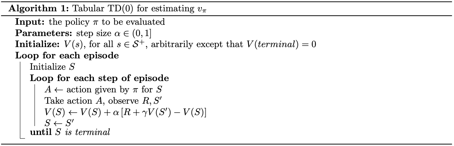
Recall that in Monte Carlo method, or even in its trivial form, constant-$\alpha$ MC, which has the update form: \begin{equation} V(S_t)\leftarrow V(S_t)+\alpha\left[G_t-V(S_t)\right]\label{eq:tp.2}, \end{equation} we have to wait until the end of the episode, when the return $G_t$ is determined. However, with TD(0), we can do the update immediately in the next time step $t+1$.

As we can see in \eqref{eq:tp.1} and \eqref{eq:tp.2}, both TD and MC updates look ahead to a sample successor state (or state-action pair), use the value of the successor and the corresponding reward in order to update the value of the current state (or state-action pair). This kind of updates is called sample update, which differs from expected update used by DP methods in that they are based on a single sample successor rather than on a complete distribution of all possible successors.

Other than the sampling of Monte Carlo, TD methods also use the bootstrapping of DP. Because similar to DP, TD(0) is also a bootstrapping method, since the target in its update is $R_{t+1}+\gamma V(S_{t+1})$.

The quantity inside bracket in \eqref{eq:tp.1} is called TD error, denoted as $\delta$: \begin{equation} \delta_t\doteq R_{t+1}+\gamma V(S_{t+1})-V(S_t) \end{equation} If the array $V$ does not change during the episode (as in MC), then the MC error can be written as a sum of TD errors \begin{align} G_t-V(S_t)&=R_{t+1}+\gamma G_{t+1}-V(S_t)+\gamma V(S_{t+1})-\gamma V(S_{t+1}) \\ &=\delta_t+\gamma\left(G_{t+1}-V(S_{t+1})\right) \\ &=\delta_t+\gamma\delta_{t+1}+\gamma^2\left(G_{t+2}-V(S_{t+2})\right) \\ &=\delta_t+\gamma\delta_{t+1}+\gamma^2\delta_{t+2}+\dots+\gamma^{T-t-1}\delta_{T-1}+\gamma^{T-t}\left(G_T-V(S_T)\right) \\ &=\delta_t+\gamma\delta_{t+1}+\gamma^2\delta_{t+2}+\dots+\gamma^{T-t-1}\delta_{T-1}+\gamma^{T-t}(0-0) \\ &=\sum_{k=t}^{T-1}\gamma^{k-t}\delta_k \end{align}

Advantages over MC & DP

With how TD is established, these are some advantages of its over MC and DP:

• Only experience is required.
• Can be fully incremental:
  • Can make update before knowing the final outcome.
  • Requires less memory.
  • Requires less peak computation.

TD(0) does converge to $v_\pi$, in the mean for a sufficient small $\alpha$, and with probability of $1$ if $\alpha$ decreases according to the stochastic approximation condition \begin{equation} \sum_{n=1}^{\infty}\alpha_n(a)=\infty\hspace{1cm}\text{and}\hspace{1cm}\sum_{n=1}^{\infty}\alpha_n^2(a)<\infty, \end{equation} where $\alpha_n(a)$ denote the step-size parameter used to process the reward received after the $n$-th selection of action $a$.

Optimality of TD(0)

Under batch training, TD(0) converges to the optimal maximum likelihood estimate. The convergence and optimality proofs can be found in this paper.

TD Control

We begin solving the control problem with an on-policy TD method. Recall that in on-policy methods, we evaluate or improve the policy $\pi$ used to make decision.

Sarsa

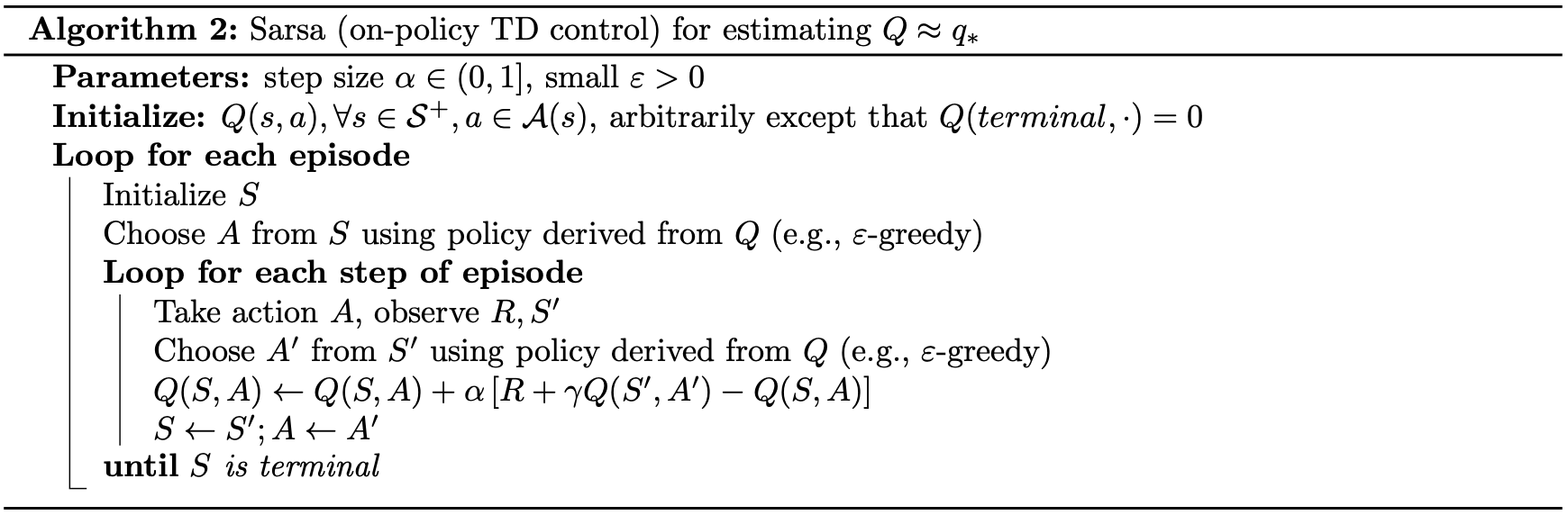
As mentioned in MC methods, when the model is not available, we have to learn an action-value function rather than a state-value function. Or in other words, we need to estimate $q_\pi(s,a)$ for the current policy $\pi$ and $\forall s,a$. Thus, instead of considering transitions from state to state in order to learn the value of states, we now take transitions from state-action pair to state-action pair into account so as to learn the value of state-action pairs.

Similarly, we’ve got the TD update for the action-value function case: \begin{equation} Q(S_t,A_t)\leftarrow Q(S_t,A_t)+\alpha\left[R_{t+1}+\gamma Q(S_{t+1},A_{t+1})-Q(S_t,A_t)\right] \end{equation} This update is done after every transition from a non-terminal state $S_t$ to its successor $S_{t+1}$ \begin{equation} \left(S_t,A_t,R_{t+1},S_{t+1},A_{t+1}\right) \end{equation} And if $S_{t+1}$ is terminal (i.e., $S_{t+1}=S_T$), then $Q(S_{t+1},A_{t+1})=0$. The name Sarsa of the method is taken based on acronym of the quintuple.

As usual when working on on-policy control problem, we apply the idea of GPI: \begin{equation} \pi_0\overset{\small \text{E}}{\rightarrow}q_{\pi_0}\overset{\small \text{I}}{\rightarrow}\pi_1\overset{\small \text{E}}{\rightarrow}q_{\pi_1}\overset{\small \text{I}}{\rightarrow}\pi_2\overset{\small \text{E}}{\rightarrow}\dots\overset{\small \text{I}}{\rightarrow}\pi_*\overset{\small \text{E}}{\rightarrow}q_* \end{equation} However this time, instead, we use it with TD methods. Which is, we continually estimate $q_\pi$ for the behavior policy $\pi$, and at the same time change $\pi$ toward greediness w.r.t $q_\pi$. That gives us the following pseudocode of the Sarsa control algorithm

Q-learning

We now turn our move to an off-policy method, which evaluates or improves a policy different from that used to generate the data.
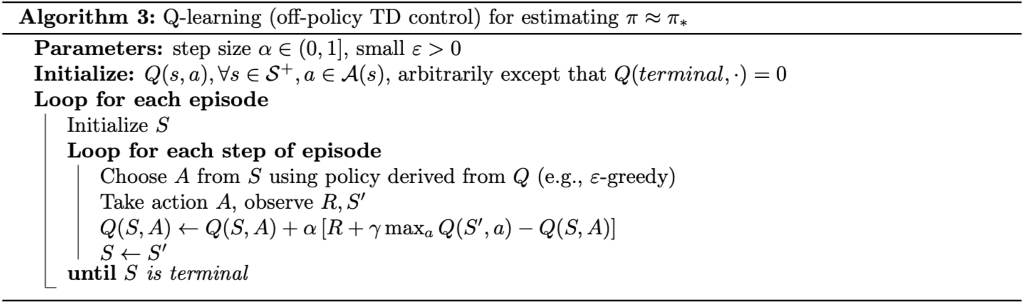
The method we are talking about is called Q-learning, which was first introduced by Watkins, in which the update on $Q$-value has the form: \begin{equation} Q(S_t,A_t)\leftarrow Q(S_t,A_t)+\alpha\left[R_{t+1}+\gamma\max_a Q(S_{t+1},a)-Q(S_t,A_t)\right]\label{eq:ql.1} \end{equation} In this case, the learned action-value function, $Q$, directly approximates optimal action-value function $q_*$, independent of the policy being followed. Down below is pseudocode of the Q-learning.

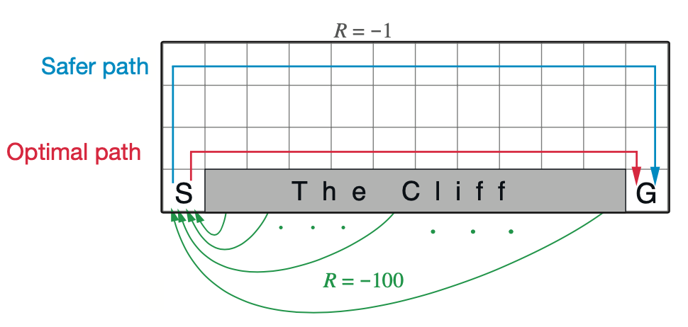
Example: Cliffwalking - Sarsa vs Q-learning

(This example is taken from Example 6.6, Reinforcement Learning: An Introduction book.)

Solution
The source code can be found here.

We begin by importing necessary packages we will be using

import numpy as np
import matplotlib.pyplot as plt
from tqdm import tqdm

Our first step is to define the environment, gridworld with a cliff, which is constructed by height, width, cliff region, start state, goal state, actions and rewards.

class GridWorld:

    def __init__(self, height, width, start_state, goal_state, cliff):
        '''
        Initialization function

        Params
        ------
        height: int
            gridworld's height
        width: int
            gridworld's width
        start_state: [int, int]
            gridworld's start state
        goal_state: [int, int]
            gridworld's goal state
        cliff: list<[int, int]>
            gridworld's cliff region
    	'''
        self.height = height
        self.width = width
        self.start_state = start_state
        self.goal_state = goal_state
        self.cliff = cliff
        self.actions = [(-1, 0), (1, 0), (0, 1), (0, -1)]
        self.rewards = {'cliff': -100, 'non-cliff': -1}

The gridworld also needs some helper functions. is_terminal() function checks whether the current state is the goal state; take_action() takes an state and action as inputs and returns next state and corresponding reward while get_action_idx() gives us the index of action from action list. Putting all these functions inside GridWorld’s body, we have:

    def is_terminal(self, state):
        '''
        Whether state @state is the goal state

        Params
        ------
        state: [int, int]
            current state
        '''
        return state == self.goal_state


    def take_action(self, state, action):
        '''
        Take action @action at state @state

        Params
        ------
        state: [int, int]
            current state
        action: (int, int)
            action taken

        Return
        ------
        (next_state, reward): ([int, int], int)
            a tuple of next state and reward
        '''
        next_state = [state[0] + action[0], state[1] + action[1]]
        next_state = [max(0, next_state[0]), max(0, next_state[1])]
        next_state = [min(self.height - 1, next_state[0]), min(self.width - 1, next_state[1])]
        if next_state in self.cliff:
            reward = self.rewards['cliff']
            next_state = self.start_state
        else:
            reward = self.rewards['non-cliff']
        return next_state, reward


    def get_action_idx(self, action):
        '''
        Get index of action in action list

        Params
        ------
        action: (int, int)
            action
        '''
        return self.actions.index(action)

Next, we define the $\varepsilon$-greedy function used by our methods in epsilon_greedy() function.

def epsilon_greedy(grid_world, epsilon, Q, state):
    '''
    Choose action according to epsilon-greedy policy

    Params:
    -------
    grid_world: GridWorld
    epsilon: float
    Q: np.ndarray
        action-value function
    state: [int, int]
        current state

    Return
    ------
    action: (int, int)
    '''
    if np.random.binomial(1, epsilon):
        action_idx = np.random.randint(len(grid_world.actions))
        action = grid_world.actions[action_idx]
    else:
        values = Q[state[0], state[1], :]
        action_idx = np.random.choice([action_ for action_, value_ 
            in enumerate(values) if value_ == np.max(values)])
        action = grid_world.actions[action_idx]
    return action

It’s time for our main course, Q-learning and Sarsa.

def q_learning(Q, grid_world, epsilon, alpha, gamma):
    '''
    Q-learning

    Params
    ------
    Q: np.ndarray
        action-value function
    grid_world: GridWorld
    epsilon: float
    alpha: float
        step size
    gamma: float
        discount factor
    '''
    state = grid_world.start_state
    rewards = 0

    while not grid_world.is_terminal(state):
        action = epsilon_greedy(grid_world, epsilon, Q, state)
        next_state, reward = grid_world.take_action(state, action)
        rewards += reward
        action_idx = grid_world.get_action_idx(action)
        Q[state[0], state[1], action_idx] += alpha * (reward + gamma * \
            np.max(Q[next_state[0], next_state[1], :]) - Q[state[0], state[1], action_idx])
        state = next_state

    return rewards

def sarsa(Q, grid_world, epsilon, alpha, gamma):
    '''
    Sarsa

    Params
    ------
    Q: np.ndarray
        action-value function
    grid_world: GridWorld
    epsilon: float
    alpha: float
        step size
    gamma: float
        discount factor
    '''
    state = grid_world.start_state
    action = epsilon_greedy(grid_world, epsilon, Q, state)
    rewards = 0

    while not grid_world.is_terminal(state):
        next_state, reward = grid_world.take_action(state, action)
        rewards += reward
        next_action = epsilon_greedy(grid_world, epsilon, Q, next_state)
        action_idx = grid_world.get_action_idx(action)
        next_action_idx = grid_world.get_action_idx(next_action)
        Q[state[0], state[1], action_idx] += alpha * (reward + gamma * Q[next_state[0], \
            next_state[1], next_action_idx] - Q[state[0], state[1], action_idx])
        state = next_state
        action = next_action

    return rewards

And lastly, wrapping everything together in the main function, we have

if __name__ == '__main__':
    height = 4
    width = 13
    start_state = [3, 0]
    goal_state = [3, 12]
    cliff = [[3, x] for x in range(1, 12)]
    grid_world = GridWorld(height, width, start_state, goal_state, cliff)
    n_runs = 50
    n_eps = 500
    epsilon = 0.1
    alpha = 0.5
    gamma = 1
    Q = np.zeros((height, width, len(grid_world.actions)))
    rewards_q_learning = np.zeros(n_eps)
    rewards_sarsa = np.zeros(n_eps)

    for _ in tqdm(range(n_runs)):
        Q_q_learning = Q.copy()
        Q_sarsa = Q.copy()

        for ep in range(n_eps):
            rewards_q_learning[ep] += q_learning(Q_q_learning, grid_world, epsilon, alpha, gamma)
            rewards_sarsa[ep] += sarsa(Q_sarsa, grid_world, epsilon, alpha, gamma)

    rewards_q_learning /= n_runs
    rewards_sarsa /= n_runs

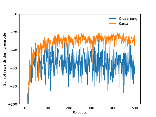
    plt.plot(rewards_q_learning, label='Q-Learning')
    plt.plot(rewards_sarsa, label='Sarsa')
    plt.xlabel('Episodes')
    plt.ylabel('Sum of rewards during episode')
    plt.ylim([-100, 0])
    plt.legend()

    plt.savefig('./cliff_walking.png')
    plt.close()

This is our result after completing running the code.

Expected Sarsa

In the update \eqref{eq:ql.1} of Q-learning, rather than taking the maximum over next state-action pairs, we use the expected value to consider how likely each action is under the current policy. That means, we instead have the following update rule for $Q$-value: \begin{align} Q(S_t,A_t)&\leftarrow Q(S_t,A_t)+\alpha\Big[R_{t+1}+\gamma\mathbb{E}_\pi\big[Q(S_{t+1},A_{t+1}\vert S_{t+1})\big]-Q(S_t,A_t)\Big] \\ &\leftarrow Q(S_t,A_t)+\alpha\Big[R_{t+1}+\gamma\sum_a\pi(a|S_{t+1})Q(S_{t+1}|a)-Q(S_t,A_t)\Big] \end{align} However, given the next state, $S_{t+1}$, this algorithms move deterministically in the same direction as Sarsa moves in expectation. Thus, this method is also called Expected Sarsa.

Expected Sarsa performs better than Sarsa since it eliminates the variance due to the randomization in selecting $A_{t+1}$. Which also means that it takes expected Sarsa more resource than Sarsa.

Double Q-learning

Maximization Bias

Consider a set of $M$ random variables $X=\{X_1,\dots,X_M\}$. Say that we are interested in maximizing expected value of the r.v.s in $X$: \begin{equation} \max_{i=1,\dots,M}\mathbb{E}(X_i)\label{eq:mb.1} \end{equation} This value can be approximated by constructing approximations for $\mathbb{E}(X_i)$ for all $i$. Let \begin{equation} S=\bigcup_{i=1}^{M}S_i \end{equation} denote a set of samples, where $S_i$ is the subset containing samples for the variables $X_i$, and assume that the samples in $S_i$ are i.i.d. Unbiased estimates for the expected values can be obtained by computing the sample average for each variable: \begin{equation} \mathbb{E}(X_i)=\mathbb{E}(\mu_i)\approx\mu_i(S)\doteq\frac{1}{\vert S_i\vert}\sum_{s\in S_i}s, \end{equation} where $\mu_i$ is an estimator for variable $X_i$. This approximation is unbiased since every sample $s\in S_i$ is an unbiased estimate for the value of $\mathbb{E}(X_i)$. Thus, \eqref{eq:mb.1} can be approximated by: \begin{equation} \max_{i=1,\dots,M}\mathbb{E}(X_i)=\max_{i=1,\dots,M}\mathbb{E}(\mu_i)\approx\max_{i=1,\dots,M}\mu_i(S) \end{equation} Let $f_i$, $F_i$ denote the PDF and CDF of $X_i$ and $f_i^\mu, F_i^\mu$ denote the PDF and CDF of $\mu_i$ respectively. Hence we have that \begin{align} \mathbb{E}(X_i)&=\int_{-\infty}^{\infty}x f_i(x)\hspace{0.1cm}dx;\hspace{0.5cm}F_i(x)=P(X_i\leq x)=\int_{-\infty}^{\infty}f_i(x)\hspace{0.1cm}dx \\ \mathbb{E}(\mu_i)&=\int_{-\infty}^{\infty}x f_i^\mu(x)\hspace{0.1cm}dx;\hspace{0.5cm}F_i^\mu(x)=P(\mu_i\leq x)=\int_{-\infty}^{\infty}f_i^\mu(x)\hspace{0.1cm}dx \end{align} With these notations, considering the maximal estimator $\mu_i$, which is distributed by some PDF $f_{\max}^{\mu}$, we have: \begin{align} F_{\max}^{\mu}&\doteq P(\max_i \mu_i\leq x) \\ &=P(\mu_1\leq x;\dots;\mu_M\leq x) \\ &=\prod_{i=1}^{M}P(\mu_i\leq x) \\ &=\prod_{i=1}^{M}F_i^\mu(x) \end{align} The value $\max_i\mu_i(S)$ is an unbiased estimate of $\mathbb{E}(\max_i\mu_i)$, which is given by \begin{align} \mathbb{E}\left(\max_i\mu_i\right) &=\int_{-\infty}^{\infty}x f_{\max}^{\mu}(x)\hspace{0.1cm}dx \\ &=\int_{-\infty}^{\infty}x\frac{d}{dx}\left(\prod_{i=1}^{M}F_i^\mu(x)\right)\hspace{0.1cm}dx \\ &=\sum_{i=1}^M\int_{-\infty}^{\infty}f_i^\mu(x)\prod_{j\neq i}^{M}F_i^\mu(x)\hspace{0.1cm}dx \end{align} However, as can be seen in \eqref{eq:mb.1}, the order of expectation and maximization is the other way around. This leads to the result that $\max_i\mu_i(S)$ is a biased estimate of $\max_i\mathbb{E}(X_i)$

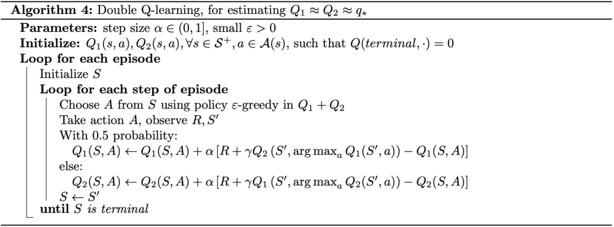
A Solution

The reason why maximization bias happens is we are using the same samples to decide which action is the best (highest reward one) and also to estimate its action-value. To overcome this situation, Hasselt (2010) proposed an alternative method that uses two set of estimators instead, $\mu^A=\{\mu_1^A,\dots,\mu_M^A\}$ and $\mu^B=\{\mu_1^B,\dots,\mu_M^B\}$. The method is thus also called double estimators.

Specifically, we use these two sets to learn two independent estimates, called $Q^A$ and $Q^B$, each is an estimate of the true value $q(a)$, for all $a\in\mathcal{A}$.

$\boldsymbol{n}$-step TD

From the definition of one-step TD, we can formalize the idea into a more general, n-step TD. Once again, first off, we will be considering the prediction problem.

$\boldsymbol{n}$-step TD Prediction

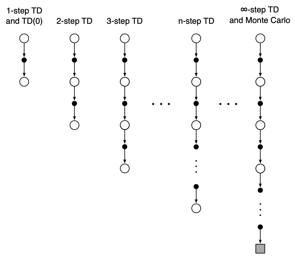
Recall that in one-step TD, the update is based on the next reward, bootstrapping² from the value of the state at one step later. In particular, the target of the update is $R_{t+1}+\gamma V_t(S_{t+1})$, which we are going to denote as $G_{t:t+1}$, or one-step return: \begin{equation} G_{t:t+1}\doteq R_{t+1}+\gamma V_t(S_{t+1}) \end{equation} where $V_t:\mathcal{S}\to\mathbb{R}$ is the estimate at time step $t$ of $v_\pi$. Thus, rather than taking into account one step later, in two-step TD, it makes sense to consider the rewards in two steps further, combined with the value function of the state at two step later. In other words, the target of two-step update is the two-step return: \begin{equation} G_{t:t+2}\doteq R_{t+1}+\gamma R_{t+2}+\gamma^2 V_{t+1}(S_{t+2}) \end{equation} Similarly, the target of $n$-step update is the $\boldsymbol{n}$-step return: \begin{equation} G_{t:t+n}\doteq R_{t+1}+\gamma R_{t+2}+\dots+\gamma^{n-1}R_{t+n}+\gamma^n V_{t+n-1}(S_{t+n}) \end{equation} for all $n,t$ such that $n\geq 1$ and $0\leq t<T-n$. If $t+n\geq T$, then all the missing terms are taken as zero, and the n-step return defined to be equal to the full return: \begin{equation} G_{t:t+n}=G_t\doteq R_{t+1}+\gamma R_{t+2}+\gamma^2 R_{t+3}+\dots+\gamma^{T-t-1}R_T,\label{eq:nstp.1} \end{equation} which is the target of the Monte Carlo update.

Hence, the $\boldsymbol{n}$-step TD method can be defined as: \begin{equation} V_{t+n}(S_t)\doteq V_{t+n-1}(S_t)+\alpha\left[G_{t:t+n}-V_{t+n-1}(S_t)\right], \end{equation} for $0\leq t<T$, while the values for all other states remain unchanged: $V_{t+n}(s)=V_{t+n-1}(s),\forall s\neq S_t$. Pseudocode of the algorithm is given right below.

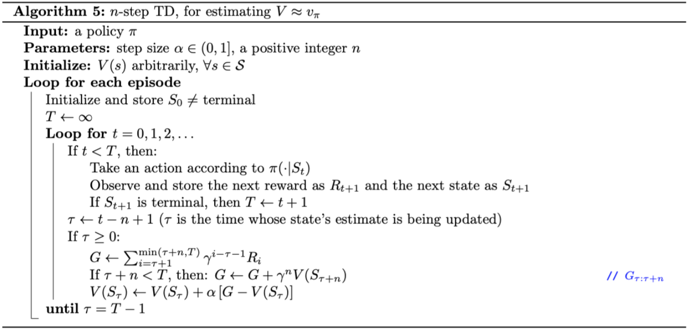
From \eqref{eq:nstp.1} combined with this definition of $n$-step TD method, it is easily seen that by changing the value of $n$ from $1$ to $\infty$, we obtain a corresponding spectrum ranging from one-step TD method to Monte Carlo method.

Example: Random Walk

(This example is taken from RL book - Example 7.1; the random process figure is created based on the one from the paper).

Suppose we have a random process as following

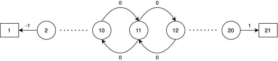
Specifically, the reward is zero everywhere except the transitions into terminal states: the transition from State 2 to State 1 (with reward of $-1$) and the transition from State 20 to State 21 (with reward of $1$). The discount factor $\gamma$ is $1$. The initial value estimates are $0$ for all states. We will implement $n$-step TD method for $n\in\{1,2,4,\dots,512\}$ and step size $\alpha\in\{0,0.2,0.4,\dots,1\}$. The walk starts at State 10.

Solution
The source code can be found here.

As usual, we need these packages for our implementation.

import numpy as np
import matplotlib.pyplot as plt
from tqdm import tqdm

First off, we need to define our environment, the random walk process. The is_terminal() function is used to check whether the state considered is a terminal state, while the take_action() function itself returns the next state and corresponding reward given the current state and the action taken.

class RandomWalk:
    '''
    Random walk environment
    '''

    def __init__(self, n_states, start_state):
        self.n_states = n_states
        self.states = np.arange(1, n_states + 1)
        self.start_state = start_state
        self.end_states = [0, n_states + 1]
        self.actions = [-1, 1]
        self.action_prob = 0.5
        self.rewards = [-1, 0, 1]


    def is_terminal(self, state):
        '''
        Whether state @state is an end state

        Params
        ------
        state: int
            current state
        '''
        return state in self.end_states


    def take_action(self, state, action):
        '''
        Take action @action at state @state

        Params
        ------
        state: int
            current state
        action: int
            action taken

        Return
        ------
        (next_state, reward): (int, int)
            a tuple of next state and reward
        '''
        next_state = state + action
        if next_state == 0:
            reward = self.rewards[0]
        elif next_state == self.n_states + 1:
            reward = self.rewards[2]
        else:
            reward = self.rewards[1]
        return next_state, reward

To calculate the RMSE, we need to compute the true value of states, which can be achieved with the help of get_true_value() function. Here we apply Bellman equations to calculate the true value of states.

def get_true_value(random_walk, gamma):
    '''
    Calculate true value of @random_walk by Bellman equations

    Params
    ------
    random_walk: RandomWalk
    gamma: float
        discount factor
    '''
    P = np.zeros((random_walk.n_states, random_walk.n_states))
    r = np.zeros((random_walk.n_states + 2, ))
    true_value = np.zeros((random_walk.n_states + 2, ))
    
    for state in random_walk.states:
        next_states = []
        rewards = []

        for action in random_walk.actions:
            next_state = state + action
            next_states.append(next_state)

            if next_state == 0:
                reward = random_walk.rewards[0]
            elif next_state == random_walk.n_states + 1:
                reward = random_walk.rewards[2]
            else:
                reward = random_walk.rewards[1]
            rewards.append(reward)

        for state_, reward_ in zip(next_states, rewards):
            if not random_walk.is_terminal(state_):
                P[state - 1, state_ - 1] = random_walk.action_prob * 1
                r[state_] = reward_
        
    u = np.zeros((random_walk.n_states, ))
    u[0] = random_walk.action_prob * 1 * (-1 + gamma * random_walk.rewards[0])
    u[-1] = random_walk.action_prob * 1 * (1 + gamma * random_walk.rewards[2])

    r = r[1:-1]
    true_value[1:-1] = np.linalg.inv(np.identity(random_walk.n_states) - gamma * P).dot(0.5 * (P.dot(r) + u))
    true_value[0] = true_value[-1] = 0

    return true_value

In this random walk experiment, we simply use random policy as our action selection.

def random_policy(random_walk):
    '''
    Choose an action randomly

    Params
    ------
    random_walk: RandomWalk
    '''
    return np.random.choice(random_walk.actions)

Now it is time to implement our algorithm.

def n_step_temporal_difference(V, n, alpha, gamma, random_walk):
    '''
    n-step TD

    Params
    ------
    V: np.ndarray
        value function
    n: int
        number of steps
    alpha: float
        step size
    random_walk: RandomWalk
    '''
    state = random_walk.start_state
    states = [state]

    T = float('inf')
    t = 0
    rewards = [0] # dummy reward to save the next reward as R_{t+1}

    while True:
        if t < T:
            action = random_policy(random_walk)
            next_state, reward = random_walk.take_action(state, action)
            states.append(next_state)
            rewards.append(reward)
            if random_walk.is_terminal(next_state):
                T = t + 1
        tau = t - n + 1 # updated state's time
        if tau >= 0:
            G = 0 # return
            for i in range(tau + 1, min(tau + n, T) + 1):
                G += np.power(gamma, i - tau - 1) * rewards[i]
            if tau + n < T:
                G += np.power(gamma, n) * V[states[tau + n]]
            if not random_walk.is_terminal(states[tau]):
                V[states[tau]] += alpha * (G - V[states[tau]])
        t += 1
        if tau == T - 1:
            break
        state = next_state

As usual, we are going illustrate our result in the main function.

if __name__ == '__main__':
    n_states = 19
    start_state = 10
    gamma = 1
    random_walk = RandomWalk(n_states, start_state)
    true_value = get_true_value(random_walk, gamma)

    episodes = 10
    runs = 100
    ns = np.power(2, np.arange(0, 10))
    alphas = np.arange(0, 1.1, 0.1)

    errors = np.zeros((len(ns), len(alphas)))
    for n_i, n in enumerate(ns):
        for alpha_i, alpha in enumerate(alphas):
            for _ in tqdm(range(runs)):
                V = np.zeros(random_walk.n_states + 2)
                for _ in range(episodes):
                    n_step_temporal_difference(V, n, alpha, gamma, random_walk)
                    rmse = np.sqrt(np.sum(np.power(V - true_value, 2) / random_walk.n_states))
                    errors[n_i, alpha_i] += rmse

    errors /= episodes * runs

    for i in range(0, len(ns)):
        plt.plot(alphas, errors[i, :], label='n = %d' % (ns[i]))
    plt.xlabel(r'$\alpha$')
    plt.ylabel('Average RMS error')
    plt.ylim([0.25, 0.55])
    plt.legend()
    plt.savefig('./random_walk.png')
    plt.close()

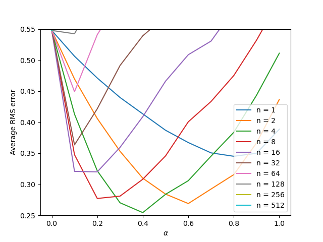
This is our result after completing running the code.

$\boldsymbol{n}$-step TD Control

Similarly, we can apply $n$-step TD methods to control task. In particular, we will combine the idea of $n$-step update with Sarsa, a control method we previously have defined above.

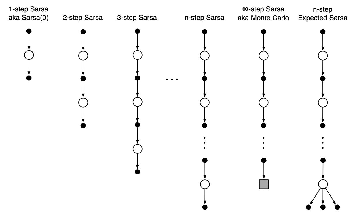
$\boldsymbol{n}$-step Sarsa

As usual, to apply our method to control problem, rather than taking into account states, we instead consider state-action pairs $s,a$ in order to learn the value functions, $q_\pi(s,a)$, of them.
Recall that the target in one-step Sarsa update is \begin{equation} G_{t:t+1}\doteq R_{t+1}+\gamma Q_t(S_{t+1},A_{t+1}) \end{equation} Similar to what we have done in the previous part of $n$-step TD Prediction, we can redefine the new target of our $n$-step update \begin{equation} G_{t:t+n}\doteq R_{t+1}+\gamma R_{t+2}+\dots+\gamma^{n-1} R_{t+n}+\gamma^n Q_{t+n-1}(S_{t+n},A_{t+n}), \end{equation} for $n\geq 0,0\leq t<T-n$, with $G_{t:t+n}\doteq G_t$ if $t+n\geq T$. The $\boldsymbol{n}$-step Sarsa is then can be defined as: \begin{equation} Q_{t+n}(S_t,A_t)\doteq Q_{t+n-1}(S_t,A_t)+\alpha\left[G_{t:t+n}-Q_{t+n-1}(S_t,A_t)\right],\hspace{1cm}0\leq t<T,\label{eq:nss.1} \end{equation} while the values of all other state-action pairs remain unchanged: $Q_{t+n}(s,a)=Q_{t+n-1}(s,a)$, for all $s,a$ such that $s\neq S_t$ or $a\neq A_t$.

From this definition of $n$-step Sarsa, we can easily derive the multiple step version of Expected Sarsa, called $\boldsymbol{n}$-step Expected Sarsa. \begin{equation} Q_{t+n}(S_t,A_t)\doteq Q_{t+n-1}(S_t,A_t)+\alpha\left[G_{t:t+n}-Q_{t+n-1}(S_t,A_t)\right],\hspace{1cm}0\leq t<T, \end{equation} which has the same rule as \eqref{eq:nss.1}, except that the target of the update in this case is defined as: \begin{equation} G_{t:t+n}\doteq R_{t+1}+\gamma R_{t+2}+\dots+\gamma^{n-1}R_{t+n}+\gamma^n\overline{V}_{t+n-1}(S_{t+n}),\hspace{1cm}t+n<T,\label{eq:nss.2} \end{equation} with $G_{t:t+n}=G_t$ for $t+n\geq T$, where $\overline{V}_t(s)$ is the expected approximate value of state $s$, using the estimated action value at time $t$, under the target policy $\pi$: \begin{equation} \overline{V}_t(s)\doteq\sum_a\pi(a|s)Q_t(s,a),\hspace{1cm}\forall s\in\mathcal{S}\label{eq:nss.3} \end{equation} If $s$ is terminal, then its expected approximate value is defined to be zero.

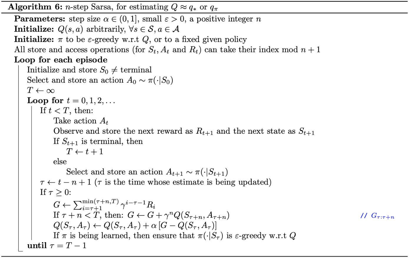
Pseudocode of the $n$-step Sarsa algorithm is given right below.

When taking the value of $n$ from $1$ to $\infty$, similarly, we also obtain a corresponding spectrum ranging from one-step Sarsa to Monte Carlo.

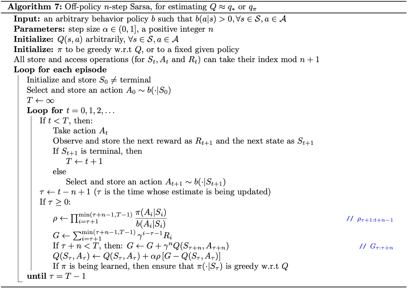
Off-policy $\boldsymbol{n}$-step TD

Recall that off-policy methods are ones that learn the value function of a target policy, $\pi$, while follows a behavior policy, $b$. In this section, we will be considering an off-policy $n$-step TD, or in specifically, $n$-step TD using Importance Sampling³.

$\boldsymbol{n}$-step TD with Importance Sampling

In $n$-step methods, returns are constructed over $n$ steps, so we are interested in the relative probability of just those $n$ actions. Thus, by weighting updates by importance sampling ratio, $\rho_{t:t+n-1}$, which is the relative probability under the two policies $\pi$ and $b$ of taking $n$ actions from $A_t$ to $A_{t+n-1}$: \begin{equation} \rho_{t:h}\doteq\prod_{k=t}^{\min(h,T-1)}\frac{\pi(A_k|S_k)}{b(A_k|S_k)}, \end{equation} we can get the off-policy $\boldsymbol{n}$-step TD method. \begin{equation} V_{t+n}(S_t)\doteq V_{t+n-1}(S_t)+\alpha\rho_{t:t+n-1}\left[G_{t:t+n}-V_{t+n-1}(S_t)\right],\hspace{1cm}0\leq t<T \end{equation} Similarly, we have the off-policy $\boldsymbol{n}$-step Sarsa method. \begin{equation} Q_{t+n}(S_t,A_t)\doteq Q_{t+n-1}(S_t,A_t)+\alpha\rho_{t:t+n-1}\left[G_{t:t+n}-Q_{t+n-1}(S_t,A_t)\right],\hspace{0.5cm}0\leq t <T\label{eq:nsti.1} \end{equation} The off-policy $\boldsymbol{n}$-step Expected Sarsa uses the same update as \eqref{eq:nsti.1} except that it uses $\rho_{t+1:t+n-1}$ as its importance sampling ratio instead of $\rho_{t+1:t+n}$ and also has \eqref{eq:nss.2} as its target.

Following is pseudocode of the off-policy $n$-step Sarsa.

Per-decision Methods with Control Variates

Recall that in the note of Monte Carlo Methods, to reduce the variance even in the absence of discounting (i.e., $\gamma=1$), we used a method called Per-decision Importance Sampling. So how about we use it with multi-step off-policy TD methods?

We begin rewriting the $n$-step return ending at horizon $h$ as: \begin{equation} G_{t:h}=R_{t+1}+\gamma G_{t+1:h},\hspace{1cm}1\lt h\lt T, \end{equation} where $G_{h:h}\doteq V_{h-1}(S_h)$.

Since we are following a policy $b$ that is not the same as the target policy $\pi$, all of the resulting experience, including the first reward $R_{t+1}$ and the next state $S_{t+1}$ must be weighted by the importance sampling ratio for time $t$, $\rho_t=\frac{\pi(A_t\vert S_t)}{b(A_t\vert S_t)}$. And moreover, to avoid the high variance when the $n$-step return is zero (resulting when the action at time $t$ would never be select by $\pi$, which leads to $\rho_t=0$), we define the $n$-step return ending at horizon $h$ for the off-policy state-value prediction as: \begin{equation} G_{t:h}\doteq\rho_t\left(R_{t+1}+\gamma G_{t+1:h}\right)+(1-\rho_t)V_{h-1}(S_t),\hspace{1cm}1\lt h\lt T\label{eq:pdcv.1} \end{equation} where $G_{h:h}\doteq V_{h-1}(S_h)$. The second term of \eqref{eq:pdcv.1}, $(1-\rho_t)V_{h-1}(S_t)$, is called control variate, which has the expected value of $0$, and then does not change the expected update.

For state-action values, the off-policy definition of the $n$-step return ending at horizon $h$ can be defined as: \begin{align} G_{t:h}&\doteq R_{t+1}+\gamma\left(\rho_{t+1}G_{t+1:h}+\overline{V}_{h-1}(S_{t+1})-\rho_{t+1}Q_{h-1}(S_{t+1},A_{t+1})\right) \\ &=R_{t+1}+\gamma\rho_{t+1}\big(G_{t+1:h}-Q_{h-1}(S_{t+1},A_{t+1})\big)+\gamma\overline{V}_{h-1}(S_{t+1}),\hspace{1cm}t\lt h\leq T\label{eq:pdcv.2} \end{align} If $h\lt T$, the recursion ends with $G_{h:h}\doteq Q_{h-1}(S_h,A_h)$, whereas, if $h\geq T$, the recursion ends with $G_{T-1:h}\doteq R_T$.

$\boldsymbol{n}$-step Tree Backup

So, is there possibly an off-policy method without the use of importance sampling? Yes, and of them is called Tree-backup.

The idea of tree-backup update is to start with the target of the one-step update, which is defined as the first reward plus the discounted estimated value of the next state. This estimated value is computed as the weighted sum of estimated action values. Each weight corresponding to an action is proportional to its probability of occurrence. In particular, the target of one-step tree-backup update is: \begin{equation} G_{t:t+1}\doteq R_{t+1}+\gamma\sum_a\pi(a|S_{t+1})Q_t(S_{t+1},a),\hspace{1cm}t<T-1 \end{equation} which is the same as that of Expected Sarsa. With two-step update, for a certain action $A_{t+1}$ taken according to the behavior policy, $b$ (i.e. $b(A_{t+1}|S_{t+1})=1$), one step later, the estimated value of the next state similarly now, can be computed as: \begin{equation} \pi(A_{t+1}|S_{t+1})\Big(R_{t+2}+\gamma\pi(a|S_{t+2})Q_{t+1}(S_{t+2},a)\Big) \end{equation} The target of two-step update, which also is defined as sum of the first reward received plus the discounted estimated value of the next state therefore, can be computed as \begin{align} G_{t:t+2}&\doteq R_{t+1}+\gamma\sum_{a\neq A_{t+1}}\pi(a|S_{t+1})Q_{t+1}(S_{t+1},a) \\ &\hspace{1cm}+\gamma\pi(A_{t+1}|S_{t+1})\Big(R_{t+2}+\gamma\pi(a|S_{t+2})Q_{t+1}(S_{t+2},a)\Big) \\&=R_{t+1}+\gamma\sum_{a\neq A_{t+1}}\pi(a|S_{t+1})Q_{t+1}(S_{t+1},a)+\gamma\pi(A_{t+1}|S_{t+1})G_{t+1:t+2}, \end{align} for $t<T-2$. Hence, the target of the $n$-step tree-backup update recursively can be defined as: \begin{equation} G_{t:t+n}\doteq R_{t+1}+\gamma\sum_{a\neq A_{t+1}}\pi(a|S_{t+1})Q_{t+n-1}(S_{t+1},a)+\gamma\pi(A_{t+1}|S_{t+1})G_{t+1:t+n}\label{eq:nstb.1} \end{equation} for $t<T-1,n\geq 2$. The $n$-step tree-backup update can be illustrated through the following diagram

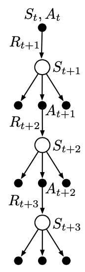
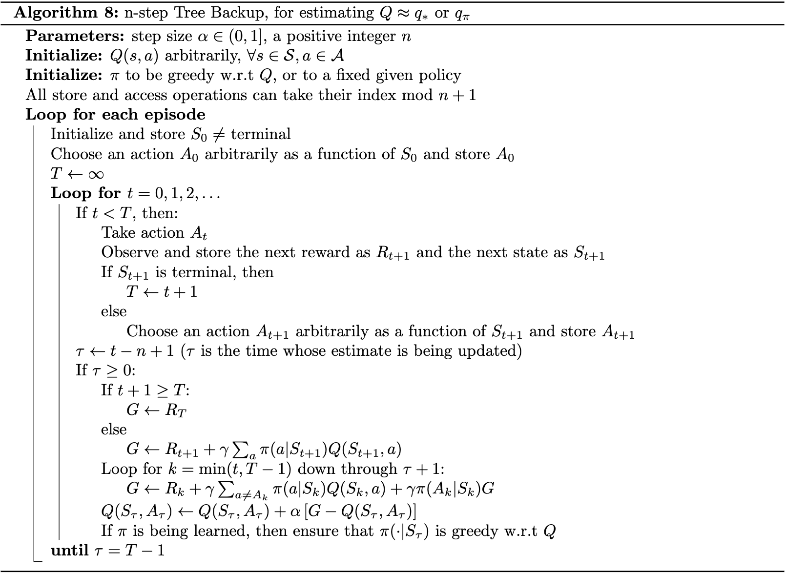
With this definition of the target, we now can define our $\boldsymbol{n}$-step tree-backup method as: \begin{equation} Q_{t+n}(S_t,A_t)\doteq Q_{t+n-1}(S_t,A_t)+\alpha\Big[G_{t:t+n}-Q_{t+n-1}(S_t,A_t)\Big],\hspace{1cm}0\leq t<T \end{equation} while the values of all other state-action pairs remain unchanged: $Q_{t+n}(s,a)=Q_{t+n-1}(s,a)$, for all $s,a$ such that $s\neq S_t$ or $a\neq A_t$. Pseudocode of the n-step tree-backup algorithm is given below.

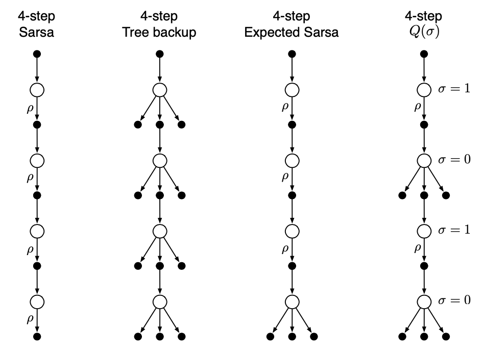
$\boldsymbol{n}$-step $Q(\sigma)$

In updating the action-value functions, if we choose always to sample, we would obtain Sarsa, whereas if we choose never to sample, we would get the tree-backup algorithm. Expected Sarsa would be the case where we choose to sample for all steps except for the last one. An possible unifying method is choosing on a state-by-state basis whether to sample or not.

We begin by rewriting the tree-backup $n$-step return \eqref{eq:nstb.1} in terms of the horizon $h=t+n$ and the expected approximate value $\overline{V}$ \eqref{eq:nss.3}: \begin{align} \hspace{-0.6cm}G_{t:h}&=R_{t+1}+\gamma\sum_{a\neq A_{t+1}}\pi(a|S_{t+1})Q_{h-1}(S_{t+1},a)+\gamma\pi(A_{t+1}|S_{t+1})G_{t+1:h} \\ &=R_{t+1}+\gamma\overline{V}_{h-1}(S_{t+1})-\gamma\pi(A_{t+1}|S_{t+1})Q_{h-1}(S_{t+1},A_{t+1})+\gamma\pi(A_{t+1}|S_{t+1})G_{t+1:h} \\ &=R_{t+1}+\gamma\pi(A_{t+1}|S_{t+1})\big(G_{t+1:h}-Q_{h-1}(S_{t+1},A_{t+1})\big)+\gamma\overline{V}_{h-1}(S_{t+1}), \end{align} which is exactly the same as the $n$-step return for Sarsa with control variates \eqref{eq:pdcv.2} except that the importance-sampling ratio $\rho_{t+1}$ has been replaced with the action probability $\pi(A_{t+1}|S_{t+1})$.

Let $\sigma_t\in[0,1]$ denote the degree of sampling on step $t$, with $\sigma=1$ denoting full sampling and $\sigma=0$ denoting a pure expectation with no sampling. The r.v $\sigma_t$ might be set as a function of the state, action or state-action pair at time $t$.

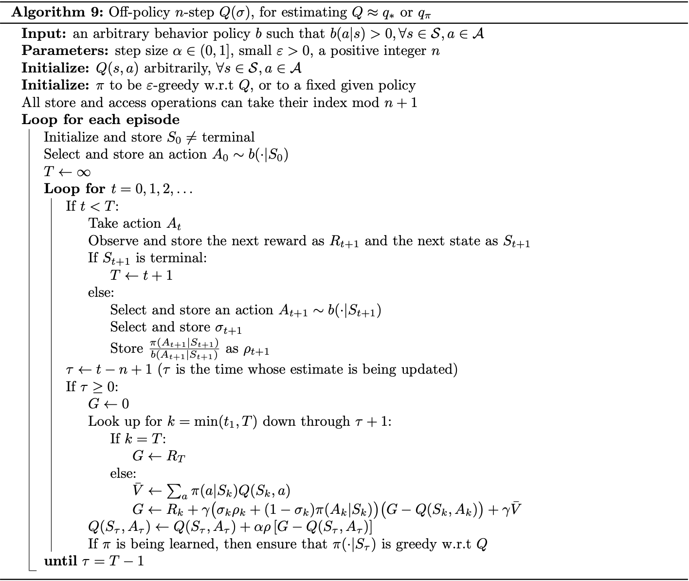
With the definition of $\sigma_t$, we can define the $n$-step return ending at horizon $h$ of the $Q(\sigma)$ as: \begin{align} G_{t:h}&\doteq R_{t+1}+\gamma\Big(\sigma_{t+1}\rho_{t+1}+(1-\rho_{t+1})\pi(A_{t+1}|S_{t+1})\Big)\Big(G_{t+1:h}-Q_{h-1}(S_{t+1},A_{t+1})\Big)\nonumber \\ &\hspace{2cm}+\gamma\overline{V}_{h-1}(S_{t+1}), \end{align} for $t\lt h\leq T$. The recursion ends with $G_{h:h}\doteq Q_{h-1}(S_h,A_h)$ if $h\lt T$, or with $G_{T-1:T}\doteq R_T$ if $h=T$. Then we use the off-policy $n$-step Sarsa update \eqref{eq:nsti.1}, which produces the pseudocode below.

References

[1] Richard S. Sutton & Andrew G. Barto. Reinforcement Learning: An Introduction. MIT press, 2018.

[2] Richard S. Sutton. Learning to predict by the methods of temporal differences. Mach Learn 3, 9–44, 1988.

[3] Chris Watkins. Learning from Delayed Rewards. PhD Thesis, 1989.

[4] Hado Hasselt. Double Q-learning. NIPS 2010.

[5] Shangtong Zhang. Reinforcement Learning: An Introduction implementation. Github.

[6] Singh, S.P., Sutton, R.S. Reinforcement learning with replacing eligibility traces. Mach Learn 22, 123–158, 1996.

Footnotes