So far in the series, we have been choosing the actions based on the estimated action value function. On the other hand, we can instead learn a parameterized policy, $\boldsymbol{\theta}$, that can select actions without consulting a value function by updating $\boldsymbol{\theta}$ on each step in the direction of an estimate of the gradient of some performance measure w.r.t $\boldsymbol{\theta}$. Such methods are called policy gradient methods.
Policy approximation
In policy gradient methods, the policy $\pi$ can be parameterized in any way, as long as $\pi(a\vert s,\boldsymbol{\theta})$ is differentiable w.r.t $\boldsymbol{\theta}$.
For discrete action space $\mathcal{A}$, a common choice of parameterization is to use parameterized numerical preferences $h(s,a,\boldsymbol{\theta})\in\mathbb{R}$ for each state-action pair. Then, the actions with the highest preferences in each state are given the highest probabilities of being selected, for instance, according to an exponential softmax distribution \begin{equation} \pi(a\vert s,\boldsymbol{\theta})\doteq\frac{e^{h(s,a,\boldsymbol{\theta})}}{\sum_b e^{h(s,b,\boldsymbol{\theta})}} \end{equation} We refer this policy approximation as softmax in action preferences.
The action preferences $h$ can be linear: \begin{equation} h(s,a,\boldsymbol{\theta})=\boldsymbol{\theta}^\text{T}\mathbf{x}(s,a), \end{equation} where $\mathbf{x}(s,a)\in\mathbb{R}^{d’}$ is the feature vector corresponding to state-action pair $(s,a)$. Or $h$ could also be calculated by a neural network.
Policy Gradient for Episodic Problems
We begin by considering episodic case, for which we define the performance measure $J(\boldsymbol{\theta})$ as the value of the start state of the episode. By assuming without loss of generality that every episode starts in some particular state $s_0$, we have: \begin{equation} J(\boldsymbol{\theta})\doteq v_{\pi_\boldsymbol{\theta}}(s_0),\label{eq:pge.1} \end{equation} where $v_{\pi_\boldsymbol{\theta}}$ is the true value function for $\pi_\boldsymbol{\theta}$, the policy parameterized by $\boldsymbol{\theta}$.
In policy gradient methods, our goal is to learn a policy $\pi_{\boldsymbol{\theta}^*}$ with a parameter vector $\boldsymbol{\theta}^*$ that maximizes the performance measure $J(\boldsymbol{\theta})$. Using gradient ascent, we iteratively update $\boldsymbol{\theta}$ by \begin{equation} \boldsymbol{\theta}_{t+1}=\boldsymbol{\theta}+\alpha\nabla J(\boldsymbol{\theta}_t), \end{equation} where $\alpha>0$ is the learning rate. By \eqref{eq:pge.1}, it is noticeable that $\nabla J(\theta)$ depends on the state distribution, which generates the start state $s_0$, which is unfortunately unknown.
However, the following theorem claims that we can express the gradient $\nabla J(\boldsymbol{\theta})$ in a form not involving the state distribution.
The Policy Gradient Theorem
Theorem 1: The policy gradient theorem for the episodic case establishes that \begin{equation} \nabla_\boldsymbol{\theta}J(\boldsymbol{\theta})\propto\sum_s\mu(s)\sum_a q_\pi(s,a)\nabla_\boldsymbol{\theta}\pi(a|s,\boldsymbol{\theta}),\label{eq:pgte.1} \end{equation} where $\pi$ represents the policy corresponding to parameter vector $\boldsymbol{\theta}$.
Proof
We have that the gradient of the state-value function w.r.t $\boldsymbol{\theta}$ can be written in terms of the action-value function, for any $s\in\mathcal{S}$, as:
\begin{align}
\hspace{-1.2cm}\nabla_\boldsymbol{\theta}v_\pi(s)&=\nabla_\boldsymbol{\theta}\Big[\sum_a\pi(a|s,\boldsymbol{\theta})q_\pi(s,a)\Big],\hspace{1cm}\forall s\in\mathcal{S} \\ &=\sum_a\Big[\nabla_\boldsymbol{\theta}\pi(a|s,\boldsymbol{\theta})q_\pi(s,a)+\pi(a|s,\boldsymbol{\theta})\nabla_\boldsymbol{\theta}q_\pi(s,a)\Big] \\ &=\sum_a\Big[\nabla_\boldsymbol{\theta}\pi(s|a)q_\pi(a,s)+\pi(a|s,\boldsymbol{\theta})\nabla_\boldsymbol{\theta}\sum_{s’,r}p(s’,r|s,a)\big(r+v_\pi(s’)\big)\Big] \\ &=\sum_a\Big[\nabla_\boldsymbol{\theta}\pi(a|s,\boldsymbol{\theta})q_\pi(s,a)+\pi(a|s,\boldsymbol{\theta})\sum_{s’}p(s’|s,a)\nabla_\boldsymbol{\theta}v_\pi(s’)\Big] \\ &=\sum_a\Big[\nabla_\boldsymbol{\theta}\pi(a|s,\boldsymbol{\theta})q_\pi(s,a)+\pi(a|s,\boldsymbol{\theta})\sum_{s’}p(s’|s,a)\sum_{a’}\big(\nabla_\boldsymbol{\theta}\pi(s’|a’,\boldsymbol{\theta})q_\pi(s’,a’) \\ &\hspace{2cm}+\pi(a’|s’,\boldsymbol{\theta})\sum_{s''}p(s''\vert s’,a’)\nabla_\boldsymbol{\theta}v_\pi(s'')\big)\Big] \\ &=\sum_{x\in\mathcal{S}}\sum_{k=0}^{\infty}P(s\to x,k,\pi)\sum_a\nabla_\boldsymbol{\theta}\pi(a|s,\boldsymbol{\theta})q_\pi(s,a),
\end{align}
After repeated unrolling as in the fifth step, where $P(s\to x,k,\pi)$ is the probability of transitioning from state $s$ to state $x$ in $k$ steps under policy $\pi$. It is then immediate that:
\begin{align}
\nabla_\boldsymbol{\theta}J(\boldsymbol{\theta})&=\nabla_\boldsymbol{\theta}v_\pi(s_0) \\ &=\sum_s\Big(\sum_{k=0}^{\infty}P(s_0\to s,k,\pi)\Big)\sum_a\nabla_\boldsymbol{\theta}\pi(a|s,\boldsymbol{\theta})q_\pi(s,a) \\ &=\sum_s\eta(s)\sum_a\nabla_\boldsymbol{\theta}\pi(a|s,\boldsymbol{\theta})q_\pi(s,a) \\ &=\sum_{s’}\eta(s’)\sum_s\frac{\eta(s)}{\sum_{s’}\eta(s’)}\sum_a\nabla_\boldsymbol{\theta}\pi(a|s,\boldsymbol{\theta})q_\pi(s,a) \\ &=\sum_{s’}\eta(s’)\sum_s\mu(s)\sum_a\nabla_\boldsymbol{\theta}\pi(a|s,\boldsymbol{\theta})q_\pi(s,a) \\ &\propto\sum_s\mu(s)\sum_a\nabla_\boldsymbol{\theta}\pi(a|s,\boldsymbol{\theta})q_\pi(s,a),
\end{align}
where $\eta(s)$ denotes the number of time steps spent, on average, in state $s$ in a single episode:
\begin{equation}
\eta(s)=h(s)+\sum_{\bar{s}}\eta(\bar{s})\sum_a\pi(a|s,\boldsymbol{\theta})p(s|\bar{s},a),\hspace{1cm}\forall s\in\mathcal{S}
\end{equation}
where $h(s)$ denotes the probability that an episode begins in each state $s$; $\bar{s}$ denotes a preceding state of $s$. This leads to the result that we have used in the fifth step:
\begin{equation}
\mu(s)=\frac{\eta(s)}{\sum_{s’}\eta(s’)},\hspace{1cm}\forall s\in\mathcal{S}
\end{equation}
REINFORCE
Notice that in Theorem 1, the right-hand side is a sum over states weighted by how often the states occur (distributed by $\mu(s)$) under the target policy $\pi$. Therefore, we can rewrite \eqref{eq:pgte.1} as: \begin{align} \nabla_\boldsymbol{\theta}J(\boldsymbol{\theta})&\propto\sum_s\mu(s)\sum_a q_\pi(s,a)\nabla_\boldsymbol{\theta}\pi(a|s,\boldsymbol{\theta}) \\ &=\mathbb{E}_\pi\left[\sum_a q_\pi(S_t,a)\nabla_\boldsymbol{\theta}\pi(a|S_t,\boldsymbol{\theta})\right]\label{eq:reinforce.1} \end{align} Using SGD on maximizing $J(\boldsymbol{\theta})$ gives us the update rule: \begin{equation} \boldsymbol{\theta}_{t+1}\doteq\boldsymbol{\theta}_t+\alpha\sum_a\hat{q}(S_t,a,\mathbf{w})\nabla_\boldsymbol{\theta}\pi(a|S_t,\boldsymbol{\theta}), \end{equation} where $\hat{q}$ is some learned approximation to $q_\pi$ with $\mathbf{w}$ denoting the weight vector of its as usual. This algorithm is called all-actions method because its update involves all of the actions.
Continue our derivation in \eqref{eq:reinforce.1}, we have: \begin{align} \nabla_\boldsymbol{\theta}J(\boldsymbol{\theta})&=\mathbb{E}_\pi\left[\sum_a q_\pi(S_t,a)\nabla_\boldsymbol{\theta}\pi(a|S_t,\boldsymbol{\theta})\right] \\ &=\mathbb{E}_\pi\left[\sum_a\pi(a|S_t,\boldsymbol{\theta})q_\pi(S_t,a)\frac{\nabla_\boldsymbol{\theta}\pi(a|S_t,\boldsymbol{\theta})}{\pi(a|S_t,\boldsymbol{\theta})}\right] \\ &=\mathbb{E}_\pi\left[q_\pi(S_t,A_t)\frac{\nabla_\boldsymbol{\theta}\pi(A_t|S_t,\boldsymbol{\theta})}{\pi(A_t|S_t,\boldsymbol{\theta}}\right] \\ &=\mathbb{E}_\pi\left[G_t\frac{\nabla_\boldsymbol{\theta}\pi(A_t|S_t,\boldsymbol{\theta})}{\pi(A_t|S_t,\boldsymbol{\theta})}\right], \end{align} where $G_t$ is the return as usual; in the third step, we have replaced $a$ by the sample $A_t\sim\pi$; and in the fourth step, we have used the identity \begin{equation} \mathbb{E}_\pi\left[G_t|S_t,A_t\right]=q_\pi(S_t,A_t) \end{equation} With this gradient, we have the SGD update for time step $t$, called the REINFORCE update, is then: \begin{equation} \boldsymbol{\theta}_{t+1}\doteq\boldsymbol{\theta}_t+\alpha G_t\frac{\nabla_\boldsymbol{\theta}\pi(A_t|S_t,\boldsymbol{\theta})}{\pi(A_t|S_t,\boldsymbol{\theta})}\label{eq:reinforce.2} \end{equation} Pseudocode of the algorithm is given below.
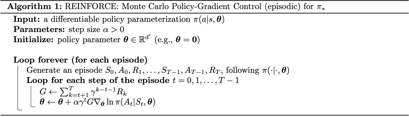
The vector \begin{equation} \frac{\nabla_\boldsymbol{\theta}\pi(a|s,\boldsymbol{\theta})}{\pi(a|s,\boldsymbol{\theta})}=\nabla_\boldsymbol{\theta}\log\pi(a|s,\boldsymbol{\theta}) \end{equation} in \eqref{eq:reinforce.2} is called the eligibility vector.
Consider using soft-max in action preferences with linear action preferences, which means that: \begin{equation} \pi(a|s,\boldsymbol{\theta})\doteq\dfrac{\exp\Big[h(s,a,\boldsymbol{\theta})\Big]}{\sum_b\exp\Big[h(s,b,\boldsymbol{\theta})\Big]}, \end{equation} where the preferences $h(s,a,\boldsymbol{\theta})$ is defined as: \begin{equation} h(s,a,\boldsymbol{\theta})=\boldsymbol{\theta}^\text{T}\mathbf{x}(s,a) \end{equation} Using the chain rule we can rewrite the eligibility vector as: \begin{align} \nabla_\boldsymbol{\theta}\log\pi(a|s,\boldsymbol{\theta})&=\nabla_\boldsymbol{\theta}\log{\frac{\exp\Big[\boldsymbol{\theta}^\text{T}\mathbf{x}(s,a)\Big]}{\sum_b\exp\Big[\boldsymbol{\theta}^\text{T}\mathbf{x}(s,b)\Big]}} \\ &=\nabla_\boldsymbol{\theta}\Big(\boldsymbol{\theta}^\text{T}\mathbf{x}(s,a)\Big)-\nabla_\boldsymbol{\theta}\log\sum_b\exp\Big[\boldsymbol{\theta}^\text{T}\mathbf{x}(s,b)\Big] \\ &=\mathbf{x}(s,a)-\dfrac{\sum_b\exp\Big[\boldsymbol{\theta}^\text{T}\mathbf{x}(s,b)\Big]\mathbf{x}(s,b)}{\sum_{b’}\exp\Big[\boldsymbol{\theta}^\text{T}\mathbf{x}(s,b’)\Big]} \\ &=\mathbf{x}(s,a)-\sum_b\pi(b|s,\boldsymbol{\theta})\mathbf{x}(s,b) \end{align}
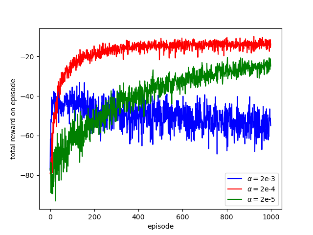
A result when using REINFORCE to solve the short-corridor problem (RL book, Example 13.1) is shown below.
REINFORCE with Baseline
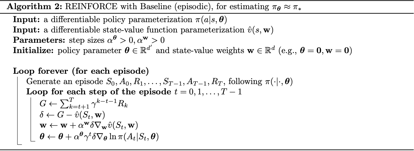
The policy gradient theorem \eqref{eq:pgte.1} can be generalized to include a comparison of the action value to an arbitrary baseline $b(s)$: \begin{equation} \nabla_\boldsymbol{\theta}J(\boldsymbol{\theta})\propto\sum_s\mu(s)\sum_a\Big(q_\pi(s,a)-b(s)\Big)\nabla_\boldsymbol{\theta}\pi(a|s,\boldsymbol{\theta}) \end{equation} The baseline can be any function, even a r.v, as long as it is independent with $a$. The equation is valid because: \begin{align} \sum_a b(s)\nabla_\boldsymbol{\theta}\pi(a|s,\boldsymbol{\theta})&=b(s)\nabla_\boldsymbol{\theta}\sum_a\pi(a|s,\boldsymbol{\theta}) \\ &=b(s)\nabla_\boldsymbol{\theta}1=0 \end{align} Using the derivation steps analogous to REINFORCE, we end up with another version of REINFORCE that includes a general baseline: \begin{equation} \boldsymbol{\theta}_{t+1}\doteq\boldsymbol{\theta}_t+\alpha\Big(G_t-b(s)\Big)\frac{\nabla_\boldsymbol{\theta}\pi(A_t|S_t,\boldsymbol{\theta})}{\pi(A_t|S_t,\boldsymbol{\theta})}\label{eq:rb.1} \end{equation} One natural baseline choice is the estimate of the state value, $\hat{v}(S_t,\mathbf{w})$, with $\mathbf{w}\in\mathbb{R}^d$ is the weight vector of its. Using this baseline, we have pseudocode of the generalization with baseline of REINFORCE algorithm \eqref{eq:rb.1} given below.
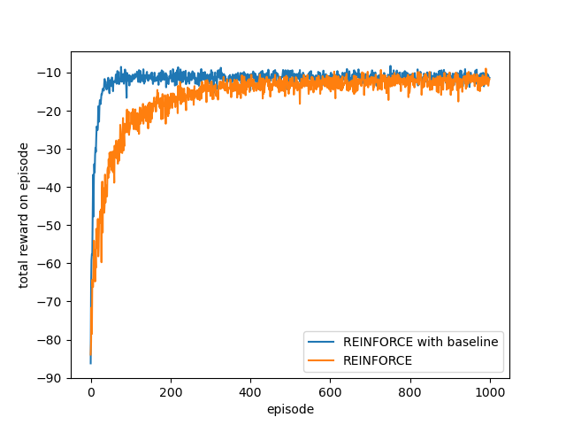
Adding a baseline to REINFORCE lets the agent learn much faster, as illustrated in the following figure.
Actor-Critic Methods
In Reinforcement Learning, methods that learn both policy and value function at the same time are called actor-critic methods, in which actor refers to the learned policy and critic is a reference to the learned value function. Although the REINFORCE with Baseline method in the previous section learns both policy and value function, but it is not an actor-critic method. Because its state-value function is used as a baseline, not as a critic, which is used for bootstrapping.
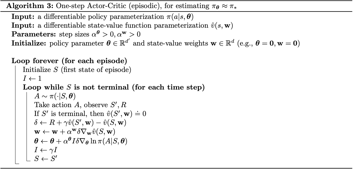
We begin by considering one-step actor-critic methods. One-step actor-critic methods replace the full return, $G_t$, of REINFORCE \eqref{eq:rb.1} with the one-step return, $G_{t:t+1}$: \begin{align} \boldsymbol{\theta}_{t+1}&\doteq\boldsymbol{\theta}_t+\alpha\Big(G_{t:t+1}-\hat{v}(S_t,\mathbf{w})\Big)\frac{\nabla_\boldsymbol{\theta}\pi(A_t|S_t,\boldsymbol{\theta})}{\pi(A_t|S_t,\boldsymbol{\theta})}\label{eq:acm.1} \\ &=\boldsymbol{\theta}_t+\alpha\Big(R_{t+1}+\hat{v}(S_{t+1},\mathbf{w})-\hat{v}(S_t,\mathbf{w})\Big)\frac{\nabla_\boldsymbol{\theta}\pi(A_t|S_t,\boldsymbol{\theta})}{\pi(A_t|S_t,\boldsymbol{\theta})} \\ &=\boldsymbol{\theta}_t+\alpha\delta_t\frac{\nabla_\boldsymbol{\theta}\pi(A_t|S_t,\boldsymbol{\theta})}{\pi(A_t|S_t,\boldsymbol{\theta})} \end{align} The natural state-value function learning method to pair with this is semi-gradient TD(0), which produces the pseudocode given below.
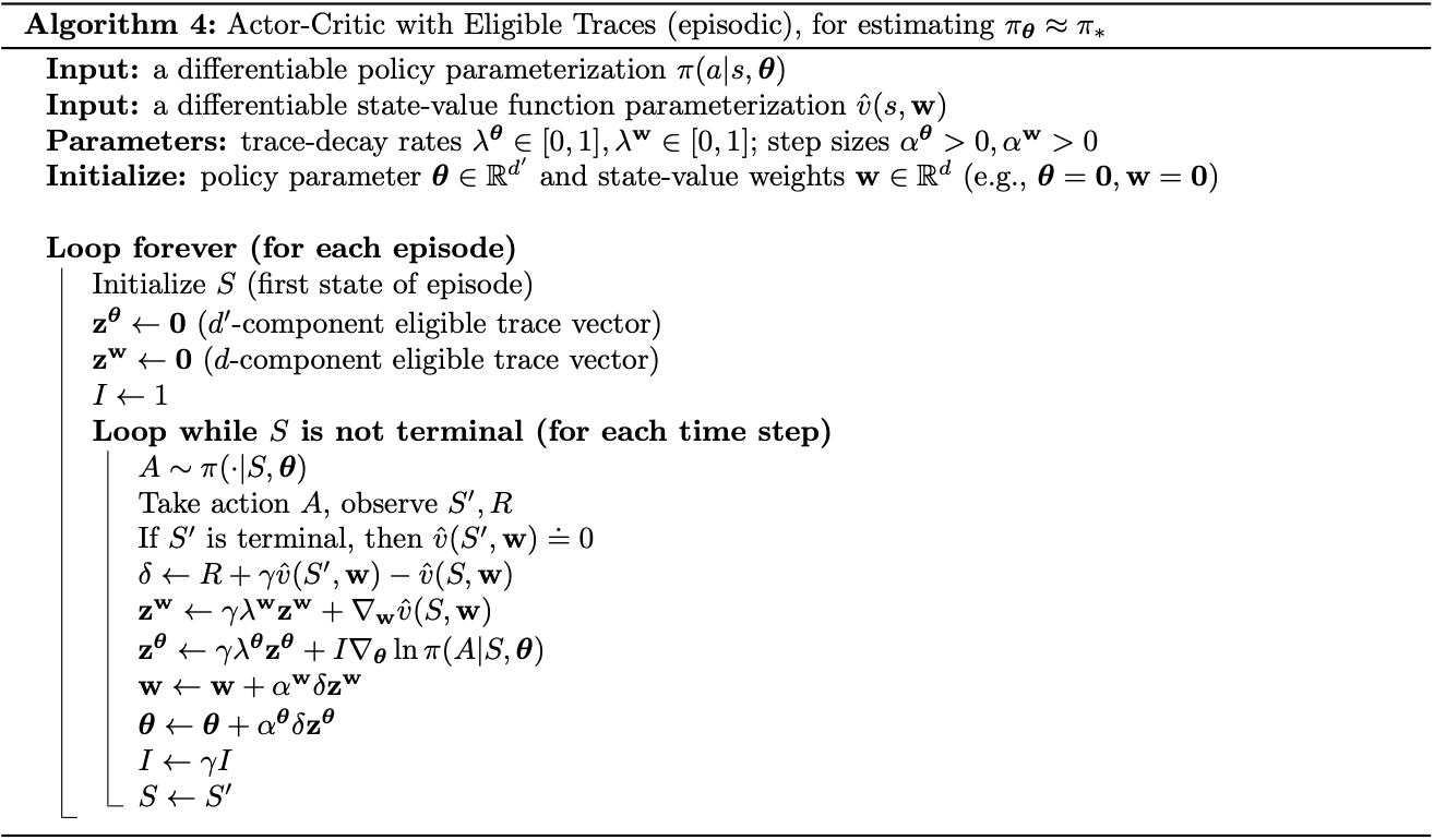
To generalize the one-step methods to the forward view of $n$-step methods and then to $\lambda$-return, in \eqref{eq:acm.1}, we simply replace the one-step return, $G_{t+1}$, by the $n$-step return, $G_{t:t+n}$, and the $\lambda$-return, $G_t^\lambda$, respectively.
In order to obtain the backward view of the $\lambda$-return algorithm, we use separately eligible traces for the actor and critic, as in the pseudocode given below.
Policy Gradient with Continuing Problems
In the continuing tasks, we define the performance measure in terms of average-reward, as: \begin{align} J(\boldsymbol{\theta})\doteq r(\pi)&\doteq\lim_{h\to\infty}\frac{1}{h}\sum_{t=1}^{h}\mathbb{E}\Big[R_t\big|S_0,A_{0:1}\sim\pi\Big] \\ &=\lim_{t\to\infty}\mathbb{E}\Big[R_t|S_0,A_{0:1}\sim\pi\Big] \\ &=\sum_s\mu(s)\sum_a\pi(a|s)\sum_{s’,r}p(s’,r|s,a)r, \end{align} where $\mu$ is the steady-state distribution under $\pi$, $\mu(s)\doteq\lim_{t\to\infty}P(S_t=s|A_{0:t}\sim\pi)$ which is assumed to exist and to be independent of $S_0$; and we also have that: \begin{equation} \sum_s\mu(s)\sum_a\pi(a|s,\boldsymbol{\theta})p(s’|s,a)=\mu(s’),\hspace{1cm}\forall s’\in\mathcal{S} \end{equation} Recall that in continuing tasks with average-reward setting, we use the differential return, which is defined in terms of differences between rewards and the average reward: \begin{equation} G_t\doteq R_{t+1}-r(\pi)+R_{t+2}-r(\pi)+R_{t+3}-r(\pi)+\dots\label{eq:pgc.1} \end{equation} And thus, we also use the differential version of value functions, which are defined as usual except that they use the differential return \eqref{eq:pgc.1}: \begin{align} v_\pi(s)&\doteq\mathbb{E}_\pi\left[G_t|S_t=s\right] \\ q_\pi(s,a)&\doteq\mathbb{E}_\pi\left[G_t|S_t=s,A_t=s\right] \end{align}
The Policy Gradient Theorem
Theorem 2: The policy gradient theorem for continuing case with average-reward states that \begin{equation} \nabla_\boldsymbol{\theta}J(\boldsymbol{\theta})=\sum_s\mu(s)\sum_a\nabla_\boldsymbol{\theta}\pi(a|s)q_\pi(s,a) \end{equation}
Proof
We have that the gradient of the state-value function w.r.t $\boldsymbol{\theta}$ can be written, for any $s\in\mathcal{S}$, as:
\begin{align}
\hspace{-1cm}\nabla_\boldsymbol{\theta}v_\pi(s)&=\boldsymbol{\theta}\Big[\sum_a\pi(a|s,\boldsymbol{\theta})q_\pi(s,a)\Big],\hspace{1cm}\forall s\in\mathcal{S} \\ &=\sum_a\Big[\nabla_\boldsymbol{\theta}\pi(a|s,\boldsymbol{\theta})q_\pi(s,a)+\pi(a|s,\boldsymbol{\theta})\nabla_\boldsymbol{\theta}q_\pi(s,a)\Big] \\ &=\sum_a\Big[\nabla_\boldsymbol{\theta}\pi(a|s,\boldsymbol{\theta})q_\pi(s,a)+\pi(a|s,\boldsymbol{\theta})\nabla_\boldsymbol{\theta}\sum_{s’,r}p(s’,r|s,a)\big(r-r(\boldsymbol{\theta})+v_\pi(s’)\big)\Big] \\ &=\sum_a\Bigg[\nabla_\boldsymbol{\theta}\pi(a|s,\boldsymbol{\theta})q_\pi(s,a)+\pi(a|s,\boldsymbol{\theta})\Big[-\nabla_\boldsymbol{\theta}r(\boldsymbol{\theta})+\sum_{s’}p(s’|s,a)\nabla_\boldsymbol{\theta}v_\pi(s’)\Big]\Bigg]
\end{align}
Thus, the gradient of the performance measure w.r.t $\boldsymbol{\theta}$ is:
\begin{align}
\hspace{-1cm}\nabla_\boldsymbol{\theta}J(\boldsymbol{\theta})&=\nabla_\boldsymbol{\theta}r(\boldsymbol{\theta}) \\ &=\sum_a\Big[\nabla_\boldsymbol{\theta}\pi(a|s,\boldsymbol{\theta})q_\pi(s,a)+\pi(a|s,\boldsymbol{\theta})\sum_{s’}p(s’|s,a)\nabla_\boldsymbol{\theta}v_\pi(s’)\Big]-\nabla_\boldsymbol{\theta}v_\pi(s) \\ &=\sum_s\mu(s)\Bigg(\sum_a\Big[\nabla_\boldsymbol{\theta}\pi(a|s,\boldsymbol{\theta})q_\pi(s,a)\nonumber \\ &\hspace{2cm}+\pi(a|s,\boldsymbol{\theta})\sum_{s’}p(s’|s,a)\nabla_\boldsymbol{\theta}v_\pi(s’)\Big]-\nabla_\boldsymbol{\theta}v_\pi(s)\Bigg) \\ &=\sum_s\mu(s)\sum_a\nabla_\boldsymbol{\theta}\pi(a|s,\boldsymbol{\theta})q_\pi(s,a)\nonumber \\ &\hspace{2cm}+\sum_s\mu(s)\sum_a\pi(a|s,\boldsymbol{\theta})\sum_{s’}p(s’|s,a)\nabla_\boldsymbol{\theta}v_\pi(s’)-\sum_s\mu(s)\nabla_\boldsymbol{\theta}v_\pi(s) \\ &=\sum_s\mu(s)\sum_a\nabla_\boldsymbol{\theta}\pi(a|s,\boldsymbol{\theta})q_\pi(s,a)\nonumber \\ &\hspace{2cm}+\sum_{s’}\sum_s\mu(s)\sum_a\pi(a|s,\boldsymbol{\theta})p(s’|s,a)\nabla_\boldsymbol{\theta}v_\pi(s’)-\sum_s\mu(s)\nabla_\boldsymbol{\theta}v_\pi(s) \\ &=\sum_s\mu(s)\sum_a\nabla_\boldsymbol{\theta}\pi(a|s,\boldsymbol{\theta})q_\pi(s,a)+\sum_{s’}\mu(s’)\nabla_\boldsymbol{\theta}v_\pi(s’)-\sum_s\mu(s)\nabla_\boldsymbol{\theta}v_\pi(s) \\ &=\sum_s\mu(s)\sum_a\nabla_\boldsymbol{\theta}\pi(a|s,\boldsymbol{\theta})q_\pi(s,a)
\end{align}
Policy Parameterization for Continuous Actions
For tasks having continuous action space with an infinite number of actions, instead of computing learned probabilities for each action, we can learn statistics of the probability distribution.
In particular, to produce a policy parameterization, the policy can be defined as the Normal distribution over a real-valued scalar action, with mean and standard deviation given by parametric function approximators that depend on the state, as given: \begin{equation} \pi(a|s,\boldsymbol{\theta})\doteq\frac{1}{\sigma(s,\boldsymbol{\theta})\sqrt{2\pi}}\exp\left(-\frac{(a-\mu(s,\boldsymbol{\theta}))^2}{2\sigma(s,\boldsymbol{\theta})^2}\right), \end{equation} where $\mu:\mathcal{S}\times\mathbb{R}^{d’}\to\mathbb{R}$ and $\sigma:\mathcal{S}\times\mathbb{R}^{d’}\to\mathbb{R}^+$ are two parameterized function approximators.
We continue by dividing the policy’s parameter vector, $\boldsymbol{\theta}=[\boldsymbol{\theta}_\mu, \boldsymbol{\theta}_\sigma]^\text{T}$, into two parts: one part, $\boldsymbol{\theta}_\mu$, is used for the approximation of the mean and the other, $\boldsymbol{\theta}_\sigma$, is used for the approximation of the standard deviation.
The mean, $\mu$, can be approximated as a linear function, while the standard deviation, $\sigma$, must always be positive, which should be approximated as the exponential of a linear function, as: \begin{align} \mu(s,\boldsymbol{\theta})&\doteq\boldsymbol{\theta}_\mu^\text{T}\mathbf{x}_\mu(s) \\ \sigma(s,\boldsymbol{\theta})&\doteq\exp\Big(\boldsymbol{\theta}_\sigma^\text{T}\mathbf{x}_\sigma(s)\Big), \end{align} where $\mathbf{x}_\mu(s)$ and $\mathbf{x}_\sigma(s)$ are state feature vectors corresponding to each approximator.
References
[1] Richard S. Sutton & Andrew G. Barto. Reinforcement Learning: An Introduction. MIT press, 2018.
[2] Deepmind x UCL. Reinforcement Learning Lecture Series 2021. Deepmind, 2021.
[3] Richard S. Sutton & David McAllester & Satinder Singh & Yishay Mansour. Policy Gradient Methods for Reinforcement Learning with Function Approximation. NIPS 1999.