Recall that when using dynamic programming (DP) method in solving reinforcement learning problems, we required the availability of a model of the environment. Whereas with Monte Carlo methods and temporal-difference learning, the models are unnecessary. Such methods with requirement of a model like the case of DP is called model-based, while methods without using a model is called model-free. Model-based methods primarily rely on planning; and model-free methods, on the other hand, primarily rely on learning.
Models & Planning
Models
A model of the environment represents anything that an agent can use to predict responses - in particular, next state and corresponding reward - of the environment to its chosen actions.
When the model is stochastic, there are several next states and rewards corresponding, each with some probability of occurring.
- If a model produces a description of all possibilities and their probabilities, we call it distribution model. For example, consider the task of tossing coin multiple times, the distribution model will produce the probability of head and the probability of tail, which is 50% for each with a fair coin.
- On the other hand, if the model produces an individual sample (head or tail) according to the probability distribution, we call it sample model.
Both types of models above can be used to mimic or simulate experience. Given a starting state and a policy, a sample model would generate an entire episode, while a distribution model could produce all possible episodes and their probabilities. We say that the model is used to simulate the environment in order to produce simulated experience.
Planning
Planning in reinforcement learning is the process of taking a model as input then output a new policy or an improved policy for interacting with the modeled environment \begin{equation} \text{model}\hspace{0.5cm}\xrightarrow[]{\hspace{1cm}\text{planning}\hspace{1cm}}\hspace{0.5cm}\text{policy} \end{equation} There are two types of planning:
- State-space planning is a search through the state space for an optimal policy or an optimal path to a goal, with two basic ideas:
- Involving computing value functions as a key intermediate step toward improving the policy.
- Computing value functions by updates or backup applied to simulated experience. \begin{equation} \text{model}\xrightarrow[]{\hspace{1.5cm}}\text{simulated experience}\xrightarrow[]{\hspace{0.3cm}\text{backups}\hspace{0.3cm}}\text{backups}\xrightarrow[]{\hspace{1.5cm}}\text{policy} \end{equation}
- Plan-space planning is a search through the space of plans.
- Plan-space planning methods consist of evolutionary methods and partial-order planning, in which the ordering of steps is not completely determined at all states of planning.
Both learning and planning methods estimate value functions by backup operations. The difference is planning uses simulated experience generated by a model compared to the uses of simulated experience generated by the environment in learning methods. This common structure lets several ideas and algorithms can be transferred between learning and planning with some modifications in the update step.
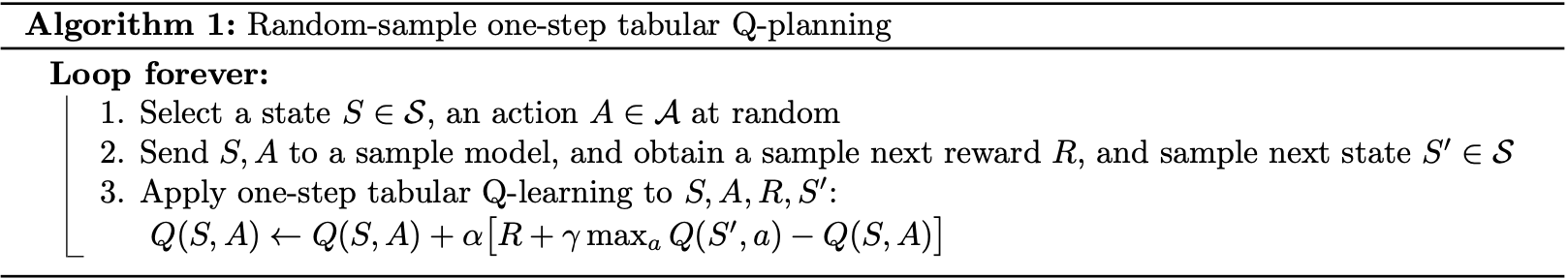
For instance, following is pseudocode of a planning method, called random-sample one-step tabular Q-planning, based on one-step tabular Q-learning, and on random samples from a sample model.
Dyna
Within a planning agent, experience plays at least two roles:
- model learning: improving the model;
- direct reinforcement learning (RL): improving the value function and policy
The figure below illustrates the possible relationships between experience, model, value functions and policy.
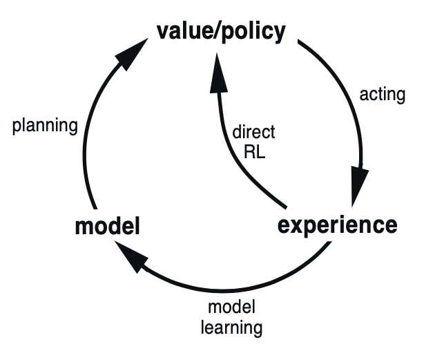
Each arrows in the diagram represents a relationship of influence and presumed improvement. It is noticeable in the diagram that experience can improve value functions and policy either directly or indirectly via model (called indirect RL), which involved in planning.
- direct RL: simpler, not affected by bad models;
- indirect RL: make fuller use of experience, i.e., getting better policy with fewer environment interactions.
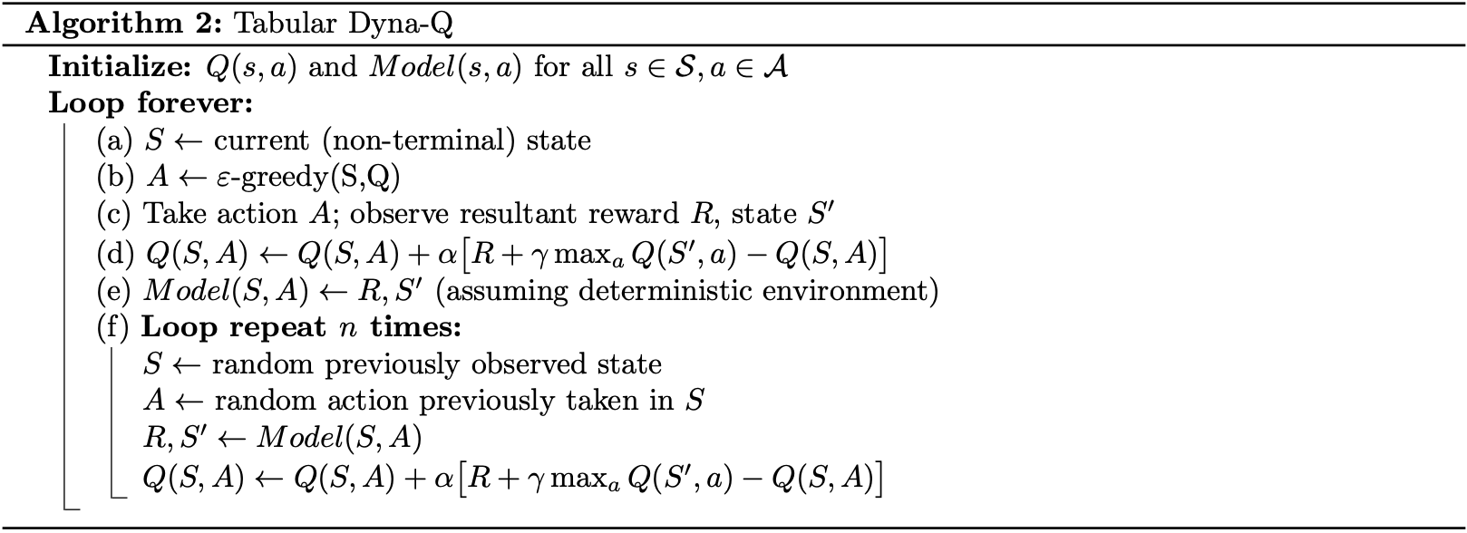
Dyna-Q
Dyna-Q is the method having all of the processes shown in the diagram in Figure 1 - planning, acting, model-learning and direct RL - all occurring continually:
- the planning method is the random-sample one-step tabular Q-planning in the previous section;
- the direct RL method is the one-step tabular Q-learning;
- the model-learning method is also table-based and assumes the environment is deterministic.
After each transition $S_t,A_t\to S_{t+1},R_{t+1}$, the model records its table entry for $S_t,A_t$ the prediction that $S_{t+1},R_{t+1}$ will deterministically follow. This lets the model simply return the last resultant next state and corresponding reward of a state-action pair when meeting them in the future.
During planning, the Q-planning algorithm randomly samples only from state-action pair that have previously been experienced. This helps the model to not be queried with a pair whose information is unknown.
Following is the general architecture of Dyna methods, of which Dyna-Q is an instance.
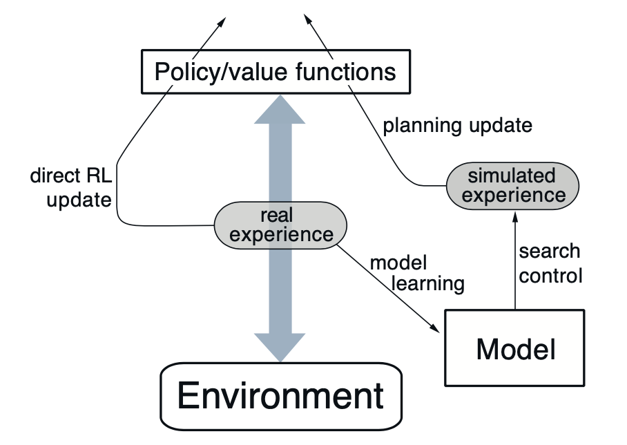
In most cases, the same reinforcement learning method is used for both learning from real experience and planning from simulated experience, which is - in this case of Dyna-Q - the Q-learning update.
Pseudocode of Dyna-Q method is shown below.
Example
(This example is taken from RL book - example 8.1.)
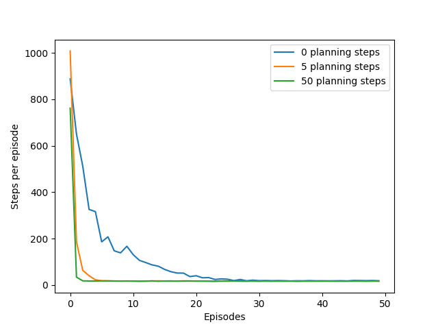
Consider a gridworld with some obstacles, called “maze” in this example, shown in the figure below.
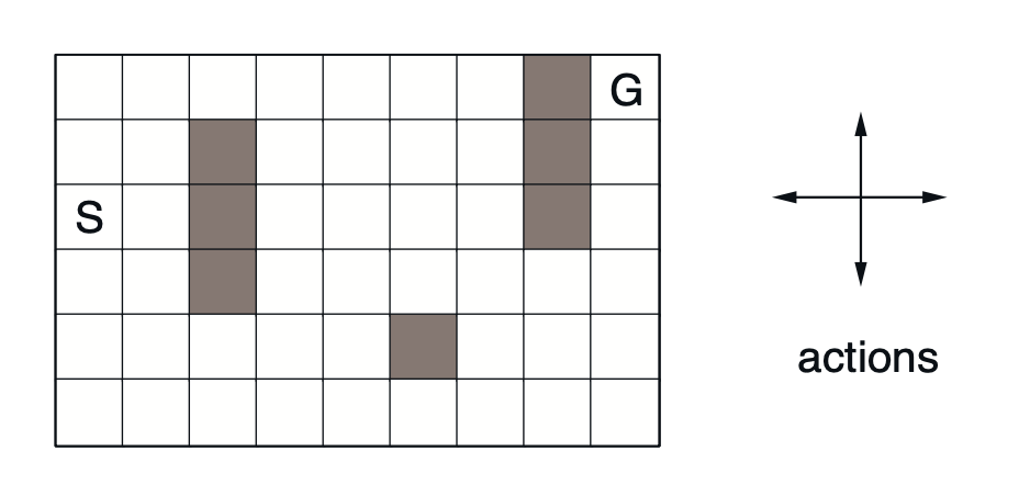
As usual, four action, $\text{up}, \text{down}, \text{right}$ and $\text{left}$ will take agent to its neighboring state, except when the agent is standing on the edge or is blocked by the obstacles, they do nothing, i.e., the agent stays still. Starting at state $S$, each transition to a non-goal state will give a reward of zero, while moving to the goal state, $G$, will reward $+1$. The episode resets when the agent reaches the goal state.
The task is discounted, episodic with $\gamma=0.95$.
Dyna-Q+
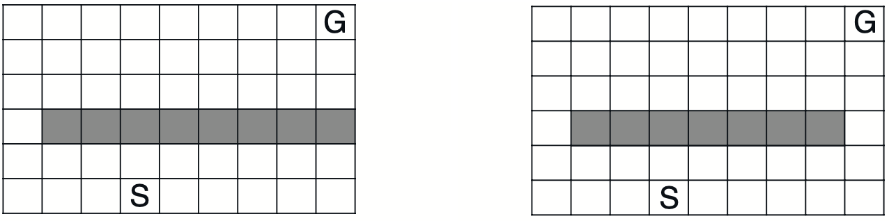
Consider a maze like the one on the left of the figure below. Suppose that after applying Dyna-Q has learned the optimal path, we make some changes to transform the gridworld into the one on the right that block the found optimal path.
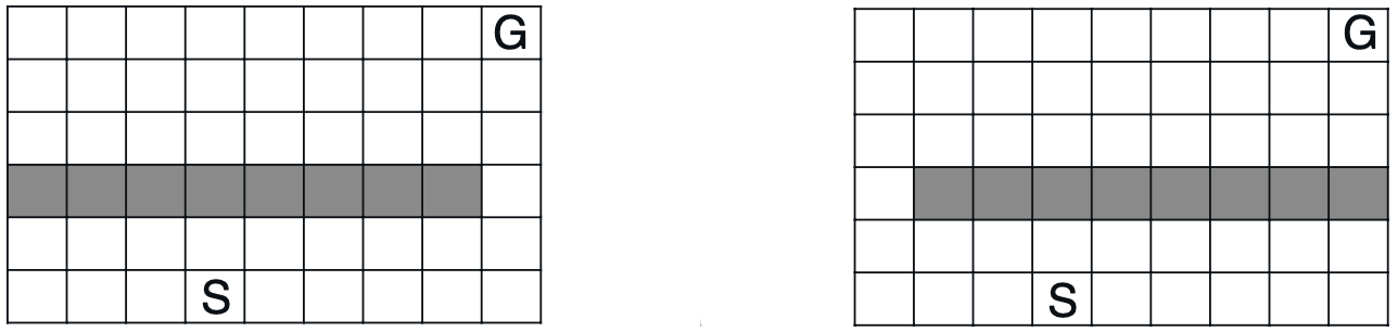
With this modification, eventually a new optimal path will be found by the Dyna-Q agent but this will takes hundreds more steps.
In this case, we want the agent to explore in order to find changes in the environment, but not so much that performance is greatly degraded. To encourage the exploration, we give it an exploration bonus:
- Keeps track for each state-action pair of how many time steps have elapsed since the pair was last tried in a real interaction with the environment.
- An special bonus reward is added for transitions caused by state-action pairs related how long ago they were tried: the long unvisited, the more reward for visiting: \begin{equation} r+\kappa\sqrt{\tau}, \end{equation} for a small (time weight) $\kappa$; where $r$ is the modeled reward for a transition; and the transition has not been tried in $\tau$ time steps.
- The agent actually plans how to visit long unvisited state-action pairs.
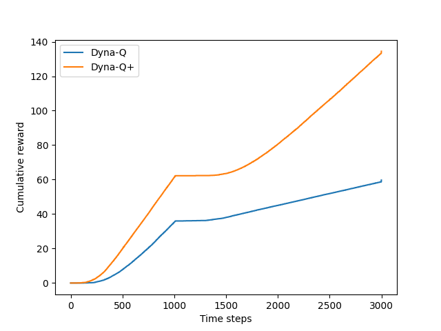
The following plot shows the performance comparison between Dyna-Q and Dyna-Q+ on this blocking task, with changing in the environment happens after 1000 steps.
We also make a comparison between with and without giving an exploration bonus to the Dyna-Q agent on the shortcut maze below.
Below is the result of using two agents solving the shortcut maze with environment modification appears after 3000 steps.
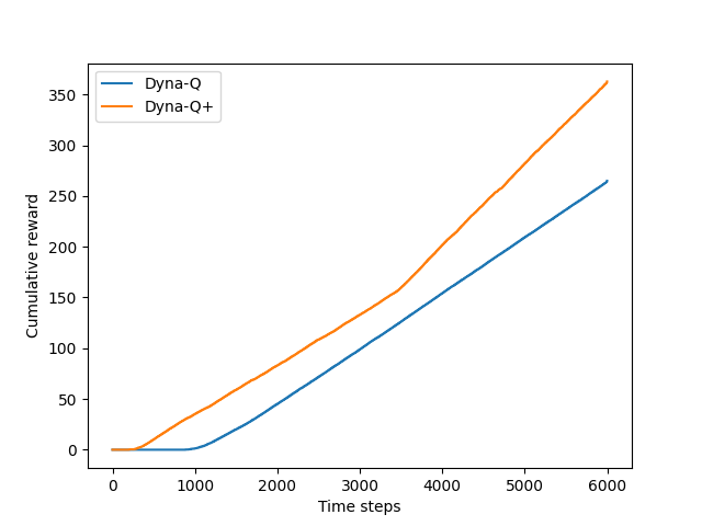
It can be seen from the plot above that the difference between Dyna-Q+ and Dyna-Q narrowed slightly over the first part of the experiment (the one using the left maze as its environment).
The reason for that is both agents were spending much more time steps than the case of blocking maze, which let the gap created by the faster convergence of Dyna-Q+ with Dyna-Q be narrowed down by exploration task, which Dyna-Q+ had to do but not Dyna-Q. This result will be more noticeable if they were stick to this first environment more time steps.
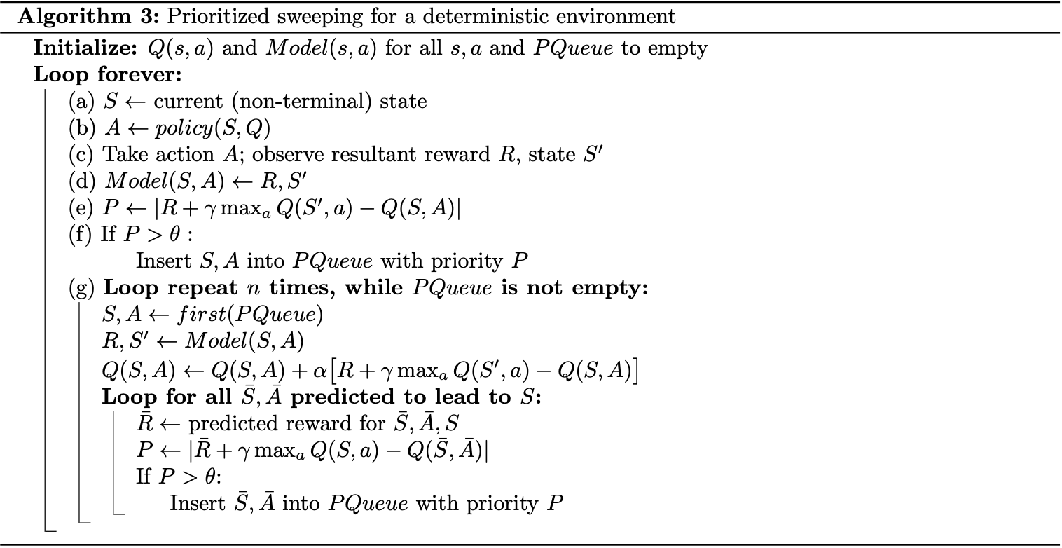
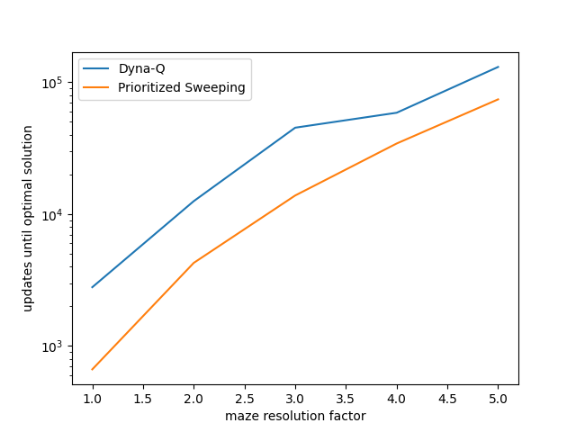
Prioritized Sweeping
Recall that in the Dyna methods presented above, the search control process selected a state-action pair randomly from all previously experienced pairs. It means that we can improve the planning if the search control instead focused on some particular state-action pairs.
Pseudocode of prioritized sweeping is shown below.
Heuristic Search
Preferences
[1] Richard S. Sutton & Andrew G. Barto. Reinforcement Learning: An Introduction. MIT press, 2018.
[2] Richard S. Sutton. Integrated Architectures for Learning, Planning, and Reacting Based on Approximating Dynamic Programming. Proceedings of the Seventh International Conference, Austin, Texas, June 21–23, 1990.
[3] Harm van Seijen & Richard S. Sutton. Efficient planning in MDPs by small backups. Proceedings of the 30th International Conference on Machine Learning (ICML 2013), 2013.
[4] Shangtong Zhang. Reinforcement Learning: An Introduction implementation. Github.