MuZero

MuZero

Predictions are made at each time step $t$, for each of $k=0,\ldots,K$ steps, by a model $\mu_\theta$, parameterized by $\theta$, conditioned on past observations $o_1,\ldots,o_t$ and on future actions $a_{t+1},\ldots,a_{t+k}$ for $k>0$.
The model $\mu_\theta$ predicts three future quantities that are directly relevant for planning:

• the policy $p_t^k\approx\pi(a_{t+k+1}\vert o_1,\ldots,o_t,a_{t+1},\ldots,a_{t+k})$;
• the value function $v_t^k\approx\mathbb{E}\big[u_{t+k+1}+\gamma u_{t+k+2}+\ldots\vert o_1,\ldots,o_t,a_{t+1},\ldots,a_{t+k}\big]$;
• the immediate reward $r_t^k\approx u_{t+k}$,

where $u$ is the true, observed reward, $\pi$ is the policy used to select real actions and $\gamma$ is the discount function of the environment.

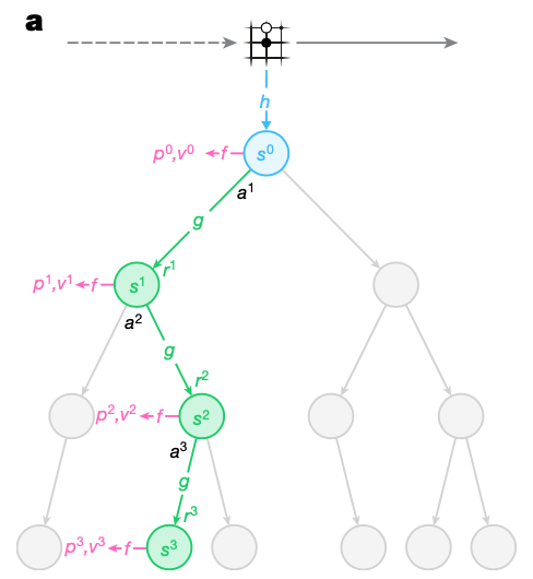
Internally, at each time step $t$, the model is represented by the combination of a representation function, a dynamics function and a prediction function.

• The (deterministic) dynamics function $g_\theta$, is a recurrent process, $(r_t^k,s_t^k)=g_\theta(s_t^{k-1},a_t^k)$, that computes, at each hypothetical step $k$, an immediate reward $r_t^k$ and an internal state $s_t^k$.
• The prediction function $f_\theta$ computes the policy and value functions from the internal state $s^k$, $(p_t^k,v_t^k)=f_\theta(s_t^k)$, similar to the joint policy and value network of AlphaZero.
• The representation function $h_\theta$ initializes the root state $s_t^0$ by encoding past observations, $s_t^0=h_\theta(o_1,\ldots,o_t)$.

Planning

Given such a model, we can apply any MDP planning algorithms, such as dynamic programming or MCTS, to compute the optimal value function or optimal policy for the MDP.

MuZero uses an MCTS algorithm similar to AlphaZero’s search (with generalized to single-agent and nonzero intermediate reward).

Search algorithm

Every node in the search tree is associated with an internal state $s$. Corresponding to each action $a$ from $s$ is an edge $(s,a)$ storing a set of statistics \begin{equation} \{N(s,a),P(s,a),Q(s,a),R(s,a),S(s,a)\} \end{equation} respectively representing visit count $N$, policy $P$, mean value $Q$, reward $R$ and state transition $S$. Analogous to AlphaZero, the algorithm iterates over three stages for a number of simulations.¹

• Selection. The stage begins at the internal root state $s^0$ and finishes when reaching a leaf node $s^l$. For each hypothetical time step $k=1,\ldots,l$ of the simulation, an action $a^k$ that maximizes over a PUCT bound is selected according to the statistics stored at $s^{k-1}$. \begin{equation} a^k=\underset{a}{\text{argmax}}\big(\bar{Q}(s^{k-1},a)+U(s^{k-1},a)\big), \end{equation} where \begin{align} \bar{Q}(s^{k-1},a)&=\frac{R(s^{k-1},a)+\gamma Q(s^{k-1},a)-\underset{s',a'\in\text{Tree}}{\min}Q(s',a')}{\underset{s',a'\in\text{Tree}}{\max}Q(s',a')-\underset{s',a'\in\text{Tree}}{\min}Q(s',a')}\label{eq:mu.1} \\ U(s^{k-1},a)&=c_\text{puct}P(s^{k-1},a)\frac{\sqrt{\sum_b N(s^{k-1},b)}}{1+N(s^{k-1},a)} \\ c_\text{puct}&=c_1+\log\frac{\sum_b N(s^{k-1},b)+c_2+1}{c_2}, \end{align} where $c_1$ and $c_2$ are constants controlling the influence of the policy $P(s^{k-1},a)$ relative to the value $Q(s^{k-1},a)$ as nodes are visited more often.
  For $k\lt l$, the next state and reward are looked up in the state transition and reward table \begin{align} s^k&=S(s^{k-1},a^k) \\ r^k&=R(s^{k-1},a^k) \end{align}
• Expansion. At the final step $l$ of the simulation, the reward and state are computed by the dynamics function $g_\theta$. \begin{equation} (r^l,s^l)=g_\theta(s^{l-1},a^l) \end{equation} and stored in the corresponding tables \begin{align} R(s^{l-1},a^l)&=r^l \\ S(s^{l-1},a^l)&=s^l \end{align} The policy and value function are computed by the prediction function $f_\theta$. \begin{equation} (p^l,v^l)=f_\theta(s^l) \end{equation} A new node, corresponding to the state $s^l$ is added to the search tree and each edge $(s^l,a)$ is initialized to \begin{equation} \{N(s^l,a)=0,Q(s^l,a)=0,P(s^l,a)=p^l\} \end{equation}
• Backup. For $k=l,\ldots,0$, we form an $(l-k)$-step estimate of the cumulative discounted reward, bootstrapping from the value function $v^l$. \begin{equation} G^k=\sum_{\tau=0}^{l-1-k}\gamma^\tau r_{k+1+\tau}+\gamma^{l-k}v^l \end{equation} The edge statistics are then updated in a backward pass through each step $k\leq l$. Specifically, for $k=l,\ldots,1$, the statistics corresponding to each edge $(s^{k-1},a^k)$ in the simulation path are updated as \begin{align} Q(s^{k-1},a^k)&\leftarrow\frac{N(s^{k-1},a^k)Q(s^{k-1},a^k)+G^k}{N(s^{k-1},a^k)+1} \\ N(s^{k-1},a^k)&\leftarrow N(s^{k-1},a^k)+1 \end{align}

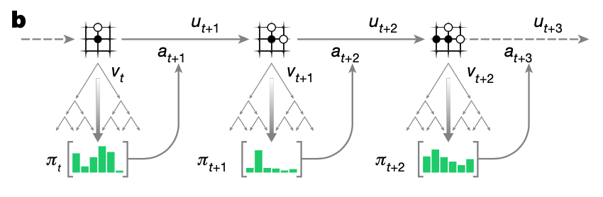
The MCTS can be viewed as a pair of a search policy and a search value function $(\pi_t,\nu_t)$ \begin{align} \pi_t&=Pr(a_{t+1}\vert o_1,\ldots,o_t) \\ \nu_t&\approx\mathbb{E}\big[u_{t+1}+\gamma u_{t+2}+\ldots\vert o_1,\ldots,o_t\big] \end{align} that both selects an action and predicts cumulative discounted reward given past observations $o_1,\ldots,o_t$. At each internal node, it makes use of the policy $p$, value function $v$ and reward estimate $G$ produced by the current model parameter $\theta$, and combines these values together using lookahead search to produce an improved policy $\pi_t$ and improved value function $\nu_t$ at the root of the search tree.

Acting

After an MCTS is performed at time step $t$, the next action $a_{t+1}$ is then selected according to the search policy $\pi_t$. With the action received, the environment generates a new observation $o_{t+1}$ and reward $u_{t+1}$. At the end of episode, the trajectory data are stored into a replay buffer.

Training

Analogy to AlphaGo Zero or AlphaZero, the self-play and network training in MuZero are executed simultaneously. The training proceeds as:

• A trajectory is sampled from the replay buffer.
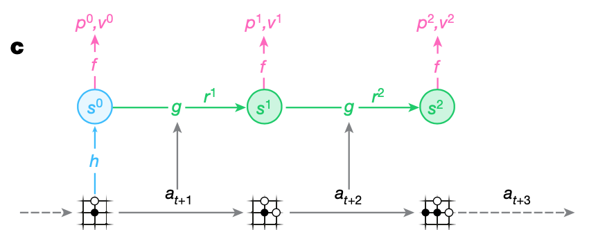
• At the initial step, the representation function $h_\theta$ produces a hidden state $s^0$ from past observations $o_1,\ldots,o_t$ from the selected trajectory.
• The model is then unrolled recurrently for $K$ steps.
• At each step $k=1,\ldots,K$, the dynamics function $g_\theta$ receives as input the hidden state $s^{k-1}$ from the previous step and the real action $a_{t+k}$.
• All parameters of the representation, dynamics and prediction functions are trained jointly, end to end, by backpropagation through time, as a single $\theta$ to match the policy $p_t^k$, value function $v_t^k$ and reward prediction $r_t^k$, for every hypothetical step $k$ to three corresponding targets observed after $k$ actual time steps have elapsed. Specifically, the overall loss used by MuZero model is \begin{equation} l_t(\theta)=\sum_{k=0}^{K}l^p(\pi_{t+k},p_t^k)+\sum_{k=0}^{K}l^v(z^{t+k},v_t^k)+\sum_{k=1}^{K}l^r(u_{t+k},r_t^k)+c\Vert\theta\Vert^2, \end{equation} where $l^p,l^v$ and $l^r$ are loss functions (e.g., cross entropy, MSE, etc) for policy, value and reward respectively; and where $\pi_t$ (recalling) is the search policy, $u_t\in\{-1,0,1\}$ is the final outcomes corresponding to {lose, draw, win} and $z_{t+k}$ is the $n$-step return that bootstraps $n$ steps into the future from the search value, i.e. $z_t=u_{t+1}+\gamma u_{t+2}+\ldots+\gamma^{n-1}u_{t+n}+\gamma^n \nu_{t+n}$.

MuZero Reanalyze

MuZero Reanalyze was proposed as a more sample efficient variant of MuZero. These following are techniques used by MuZero Reanalyze to improve its sample efficiency:

• It re-executes MCTS on past time-steps retrived from the replay buffer and uses the lastest model parameters to update the policy. This fresh policy is then potentially better than its original version.
• It ultilizes a target network to provide a fresher, stable $n$-step bootstrapped target for the value function. This value target is either computed via a simple forward path of the target network or from a MCTS rerun using the target network.

References

[1] Julian Schrittwieser, Ioannis Antonoglou, Thomas Hubert, David Silver et al. Mastering Atari, Go, chess and shogi by planning with a learned model. Nature 588, 604–609, 2020.

[2] Richard S. Sutton, Andrew G. Barto. Reinforcement Learning: An Introduction. MIT press, 2018.

[3] Julian Schrittwieser. MuZero Intuition.

Footnotes