Monte Carlo Methods in Reinforcement Learning

Recall that when using Dynamic Programming algorithms to solve RL problems, we made an assumption about the complete knowledge of the environment. With Monte Carlo methods, we only require experience - sample sequences of states, actions, and rewards from simulated or real interaction with an environment.

Monte Carlo Methods

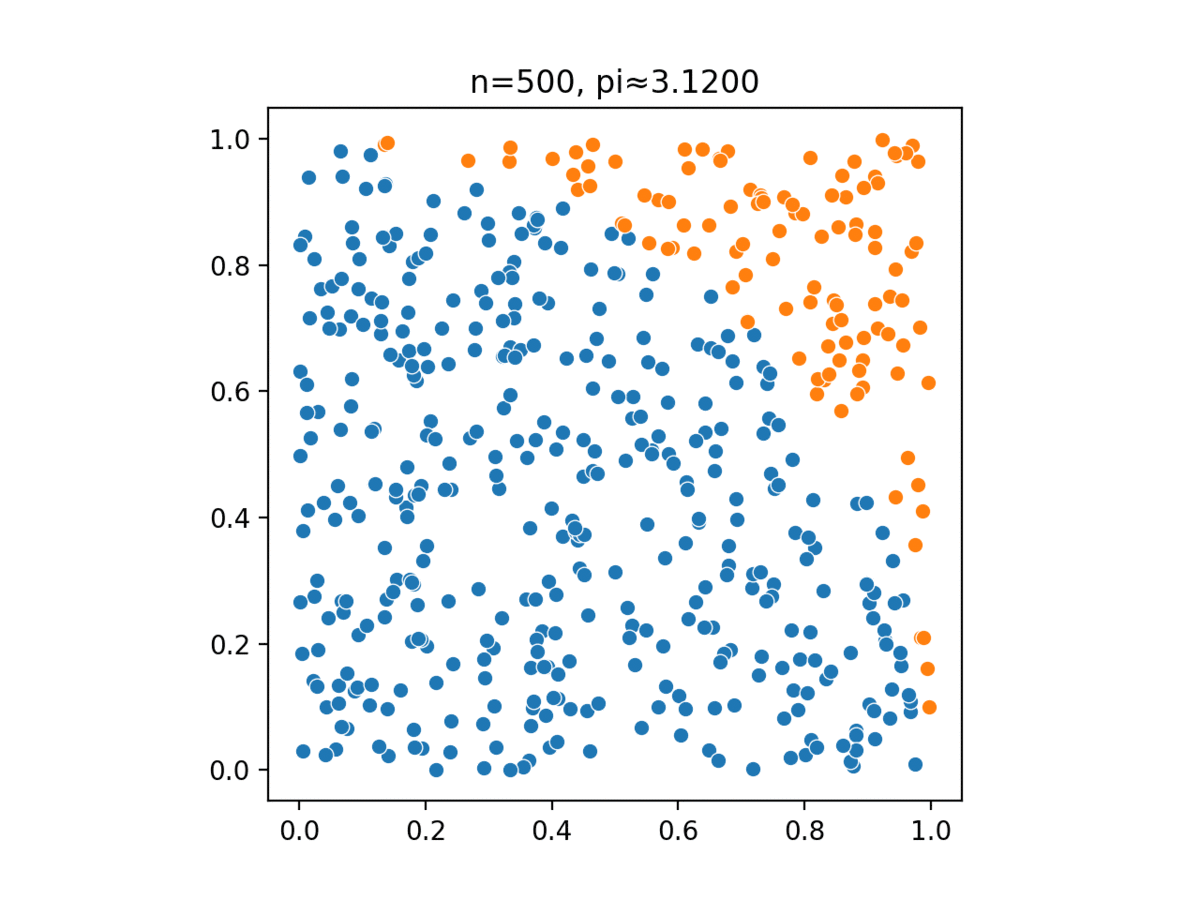
Monte Carlo, named after a casino in Monaco, simulates complex probabilistic events using simple random events, such as tossing a pair of dice to simulate the casino’s overall business model.

Monte Carlo methods have been used in several different tasks:

• Simulating a system and its probability distribution \begin{equation} x\sim\pi(x) \end{equation}
• Estimating a quantity through Monte Carlo integration \begin{equation} c=\mathbb{E}_\pi\left[f(x)\right]=\int\pi(x)f(x)\,dx \end{equation}
• Optimizing a target function to find its modes (maxima or minima) \begin{equation} x^*=\text{argmax}\,\pi(x) \end{equation}
• Learning a parameters from a training set to optimize some loss functions, such as the maximum likelihood estimation from a set of examples $\{x_i,i=1,2,\dots,M\}$ \begin{equation} \Theta^*=\text{argmax}\sum_{i=1}^{M}\log p(x_i;\Theta) \end{equation}
• Visualizing the energy landscape of a target function.

Monte Carlo Methods in Reinforcement Learning

Monte Carlo (MC) methods are ways of solving the reinforcement learning problem based on averaging sample returns. Here, we define Monte Carlo methods only for episodic tasks. Or in other words, they learn from complete episodes of experience.

Monte Carlo Prediction¹

Since the value of a state $v_\pi(s)=\mathbb{E}_\pi\left[G_t|S_t=s\right]$ is defined as the expectation of the return when the process is started from the given state $s$, an obvious way of estimating this value from experience is to compute observed mean returns after visits to that state. As more returns are observed, the average should converge to the expected value. This is an instance of the so-called Monte Carlo method.

In particular, suppose we wish to estimate $v_\pi(s)$ given a set of episodes obtained by following $\pi$ and passing through $s$. Each time state $s$ appears in an episode, we call it a visit to $s$. There are two types of Monte Carlo methods:

• First-visit MC.
  • The first time $s$ is visited in an episode is referred as the first visit to $s$.
  • The method estimates $v_\pi(s)$ as the average of the returns that have followed the first visit to $s$.
• Every-visit MC.
  • The method estimates $v_\pi(s)$ as the average of the returns that have followed all visits to to $s$.

The sample mean return for state $s$ is computed as \begin{equation} v_\pi(s)=\dfrac{\sum_{t=1}^{T}𝟙\left(S_t=s\right)G_t}{\sum_{t=1}^{T}𝟙\left(S_t=s\right)}, \end{equation} where $𝟙(\cdot)$ is an indicator function. In the case of first-visit MC, $𝟙\left(S_t=s\right)$ returns $1$ only in the first time $s$ is encountered in an episode. And for every-visit MC, $𝟙\left(S_t=s\right)$ gives value of $1$ every time $s$ is visited.

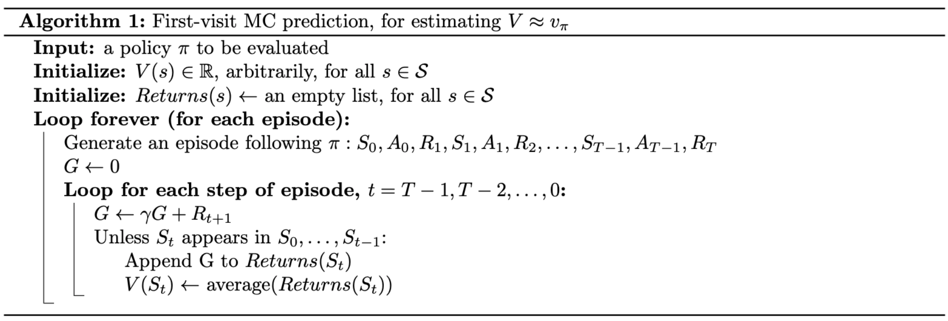
Following is pseudocode of first-visit MC prediction, for estimating $V\approx v_\pi$

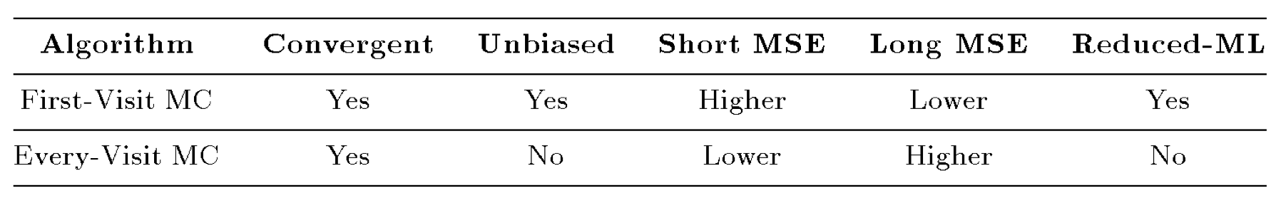
First-visit MC vs. every-visit MC

Both methods converge to $v_\pi(s)$ as the number of visits (or first visits) to $s$ goes to infinity. Each average is itself an unbiased estimate, and the standard deviation of its error falls as $\frac{1}{\sqrt{n}}$, where $n$ is the number of returns averaged.

Monte Carlo Control²

Monte Carlo Estimation of Action Values

When model is not available, it is particular useful to estimate action values rather than state values (which alone are insufficient to determine a policy). We must explicitly estimate the value of each action in order for the values to be useful in suggesting a policy. Thus, one of our primary goals for MC methods is to estimate $q_*$. To achieve this, we first consider the policy evaluation problem for action values.

Similar to when using MC method to estimate $v_\pi(s)$, we can use both first-visit MC and every-visit MC to approximate the value of $q_\pi(s,a)$. The only thing we need to keep in mind is, in this case, we work with visits to a state-action pair rather than to a state. Likewise, we define two types of MC methods for estimating $q_\pi(s,a)$:

• First-visit MC: estimates $q_\pi(s,a)$ as the average of the returns following the first time in each episode that the state $s$ was visited and the action $a$ was selected.
• Every-visit MC: estimates $q_\pi(s,a)$ as the average of the returns that have followed all the visits to state-action pair $(s,a)$.

Exploring Starts

However, here we must exercise exploration. Because many state-action pairs may never be visited, and if $\pi$ is a deterministic policy, then returns of only single one action for each state will be observed. That leads to the consequence that the other actions will not be evaluated since there are no returns to average.

There is one way to achieve this, which is called exploring starts - an assumption that assumes the episodes start in a state-action pair, and that every pair has a nonzero probability of being selected as the start. This assumption assures that all state-action pairs will be visited an infinite number of times in the limit of an infinite number of episodes.

Monte Carlo Policy Iteration

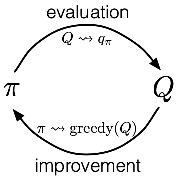
To learn the optimal policy by MC, we apply the idea of GPI: \begin{equation} \pi_0\overset{\small \text{E}}{\rightarrow}q_{\pi_0}\overset{\small \text{I}}{\rightarrow}\pi_1\overset{\small \text{E}}{\rightarrow}q_{\pi_1}\overset{\small \text{I}}{\rightarrow}\pi_2\overset{\small \text{E}}{\rightarrow}\dots\overset{\small \text{I}}{\rightarrow}\pi_*\overset{\small \text{E}}{\rightarrow}q_* \end{equation} Specifically,

1. Policy evaluation (denoted $\overset{\small\text{E}}{\rightarrow}$): estimates action value function $q_\pi(s,a)$ using the episode generated from $s, a$, following by current policy $\pi$ \begin{equation} q_\pi(s,a)=\dfrac{\sum_{t=1}^{T}𝟙\left(S_t=s,A_t=a\right)G_t}{\sum_{t=1}^{T}𝟙\left(S_t=s,A_t=a\right)} \end{equation}
2. Policy improvement (denoted $\overset{\small\text{I}}{\rightarrow}$): makes the policy greedy with the current value function (action value function in this case) \begin{equation} \pi(s)\doteq\underset{a\in\mathcal{A(s)}}{\text{argmax}},q(s,a) \end{equation} The policy improvement can be done by constructing each $\pi_{k+1}$ as the greedy policy w.r.t $q_{\pi_k}$ because \begin{align} q_{\pi_k}\left(s,\pi_{k+1}(s)\right)&=q_{\pi_k}\left(s,\underset{a}{\text{argmax}},q_{\pi_k}(s,a)\right) \\ &=\max_a q_{\pi_k}(s,a) \\ &\geq q_{\pi_k}\left(s,\pi_k(s)\right) \\ &\geq v_{\pi_k}(s) \end{align} Therefore, by the policy improvement theorem, we have that $\pi_{k+1}\geq\pi_k$.

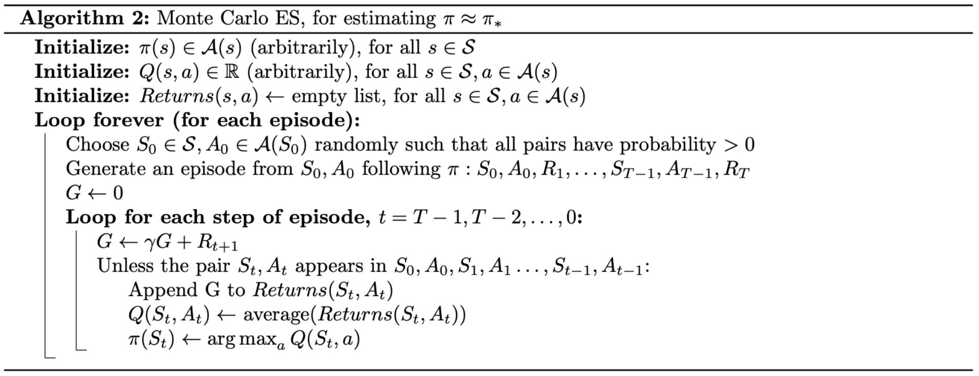
To solve this problem with Monte Carlo policy iteration, in the 1998 version of “Reinforcement Learning: An Introduction”, authors of the book introduced Monte Carlo ES (MCES), for Monte Carlo with exploring starts.

In MCES, value function is approximated by simulated returns and a greedy policy is selected at each iteration. Although MCES does not converge to any sub-optimal policy, the convergence to optimal fixed-point is still an open question. For solutions in particular settings, you can check out some results like Tsitsiklis (2002), Chen (2018), Liu (2020).
Down below is pseudocode of the Monte Carlo ES.

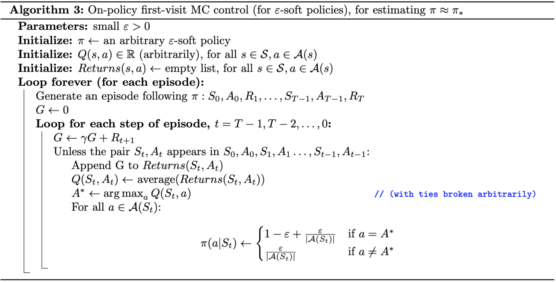
On-policy Monte Carlo Control³

In the previous section, we used the assumption of exploring starts (ES) to design a Monte Carlo control method called MCES. In this part, without making that impractical assumption, we will be talking about another Monte Carlo control method.

In on-policy control methods, the policy is generally soft (i.e. $\pi(a|s)>0,\forall s\in\mathcal{S},a\in\mathcal{A(s)}$, but gradually shifted closer and closer to a deterministic optimal policy). We can not simply improve the policy by following a greedy policy, since no exploration will take place. Then to get rid of ES, we use the on-policy MC method with $\varepsilon$-greedy policies, e.g, most of the time they choose an action that maximal estimated action value, but with probability of $\varepsilon$ they instead select an action at random. Specifically,

• $Pr(\small\textit{non-greedy action})=\dfrac{\varepsilon}{\vert\mathcal{A(s)}\vert}$
• $Pr(\small\textit{greedy action})=1-\varepsilon+\dfrac{\varepsilon}{\vert\mathcal{A(s)}\vert}$

The $\varepsilon$-greedy policies are examples of $\varepsilon$-soft policies, defined as ones for which $\pi(a\vert s)\geq\frac{\varepsilon}{\vert\mathcal{A(s)}\vert}$ for all states and actions, for some $\varepsilon>0$. Among $\varepsilon$-soft policies, $\varepsilon$-greedy policies are in some sense those that closest to greedy.

We have that any $\varepsilon$-greedy policy w.r.t $q_\pi$ is an improvement over any $\varepsilon$-soft policy is assured by the policy improvement theorem.

Proof
Let $\pi’$ be the $\varepsilon$-greedy. The conditions of the policy improvement theorem apply because for any $s\in\mathcal{S}$, we have: \begin{align} q_\pi\left(s,\pi’(s)\right)&=\sum_a\pi’(a|s)q_\pi(s,a) \\ &=\dfrac{\varepsilon}{\vert\mathcal{A}(s)\vert}\sum_a q_\pi(s,a)+(1-\varepsilon)\max_a q_\pi(s,a) \\ &\geq\dfrac{\varepsilon}{\vert\mathcal{A(s)}\vert}\sum_a q_\pi(s,a)+(1-\varepsilon)\sum_a\dfrac{\pi(a|s)-\frac{\varepsilon}{\vert\mathcal{A}(s)\vert}}{1-\varepsilon}q_\pi(s,a) \\ &=\dfrac{\varepsilon}{\vert\mathcal{A}(s)\vert}\sum_a q_\pi(s,a)+\sum_a\pi(a|s)q_\pi(s,a)-\dfrac{\varepsilon}{\vert\mathcal{A}(s)\vert}\sum_a q_\pi(s,a) \\ &=v_\pi(s) \end{align} where in the third step, we have used the fact that the latter $\sum$ is a weighted average over $q_\pi(s,a)$. Thus, by the theorem, $\pi’\geq\pi$. The equality holds when both $\pi’$ and $\pi$ are optimal policies among the $\varepsilon$-soft ones.

Pseudocode of the complete algorithm is given below.

Off-policy Monte Carlo Prediction⁴

When working with control methods, we have to solve a dilemma about exploitation and exploration. In other words, we have to evaluate a policy from episodes generated by following an exploratory policy.

A straightforward way to solve this problem is to use two different policies, one that is learned about and becomes the optimal policy, and one that is more exploratory and is used to generate behavior. The policy is being learned about is called the target policy, whereas behavior policy is the one which is used to generate behavior.

In this section, we will be considering the off-policy method on prediction task, on which both target (denoted as $\pi$) and behavior (denoted as $b$) policies are fixed and given. Particularly, we wish to estimate $v_\pi$ or $q_\pi$ from episodes retrieved from following another policy $b$, where $\pi\neq b$.

Assumption of Coverage

In order to use episodes from $b$ to estimate values for $\pi$, we require that every action taken under $\pi$ is also taken, at least occasionally, under $b$. That means, we assume that $\pi(a|s)>0$ implies $b(s|a)>0$, which leads to a result that $b$ must be stochastic, while $\pi$ may be deterministic since $\pi\neq b$. This is the assumption of coverage.

Importance Sampling

Let $X$ be a variable (or set of variables) that takes on values in some space $\textit{Val}(X)$. Importance sampling (IS) is a general approach for estimating the expectation of a function $f(x)$ relative to some distribution $P(X)$, typically called the target distribution. We can estimate this expectation by generating samples $x[1],\dots,x[M]$ from $P$, and then estimating \begin{equation} \mathbb{E}_P\left[f\right]\approx\dfrac{1}{M}\sum_{m=1}^{M}f(x[m]) \end{equation} In some cases, it might be impossible or computationally very expensive to generate samples from $P$, we instead prefer to generate samples from a different distribution, $Q$, known as the proposal distribution (or sampling distribution).

• Unnormalized Importance Sampling.
  If we generate samples from $Q$ instead of $P$, we cannot simply average the $f$-value of the samples generated. We need to adjust our estimator to compensate for the incorrect sampling distribution. The most obvious way of adjusting our estimator is based on the observation that \begin{align} \mathbb{E}_{P(X)}\left[f(X)\right]&=\sum_x f(x)P(x) \\ &=\sum_x Q(x)f(x)\dfrac{P(x)}{Q(x)} \\ &=\mathbb{E}_{Q(X)}\left[f(X)\dfrac{P(X)}{Q(X)}\right]\tag{1}\label{1} \end{align} Based on this observation \eqref{1}, we can use the standard estimator for expectations relative to $Q$. We generate a set of sample $\mathcal{D}=\{x[1],\dots,x[M]\}$ from $Q$, and then estimate: \begin{equation} \hat{\mathbb{E}}_\mathcal{D}(f)=\dfrac{1}{M}\sum_{m=1}^{M}f(x[m])\dfrac{P(x[m])}{Q(x[m])}\tag{2}\label{2}, \end{equation} where $\hat{\mathbb{E}}$ denotes empirical expectation. We call this estimator the unnormalized importance sampling estimator, this method is also often called unweighted importance sampling. The factor $\frac{P(x[m])}{Q(x[m])}$ (denoted as $w(x[m])$) can be viewed as a correction weight to the term $f(x[m])$, which we would have used had $Q$ been our target distribution.
• Normalized Importance Sampling.
  In many situations, we have that $P$ is known only up to a normalizing constant $Z$. Particularly, what we have access to is a distribution $\tilde{P}(X)=ZP(X)$. Thus, rather than to define the weights relative to $P$ as above, we define: \begin{equation} w(X)\doteq\dfrac{\tilde{P}(X)}{Q(X)} \end{equation} We have that the weight $w(X)$ is a random variable, and has expected value equal to $Z$: \begin{equation} \mathbb{E}_{Q(X)}\left[w(X)\right]=\sum_x Q(x)\dfrac{\tilde{P}(x)}{Q(x)}=\sum_x\tilde{P}(x)=Z \end{equation} Hence, this quantity is the normalizing constant of the distribution $\tilde{P}$. We can now rewrite \eqref{1} as: \begin{align} \mathbb{E}_{P(X)}\left[f(X)\right]&=\sum_x P(x)f(x) \\ &=\sum_x Q(x)f(x)\dfrac{P(x)}{Q(x)} \\ &=\dfrac{1}{Z}\sum_x Q(x)f(x)\dfrac{\tilde{P}(x)}{Q(x)} \\ &=\dfrac{1}{Z}\mathbb{E}_{Q(X)}\left[f(X)w(X)\right] \\ &=\dfrac{\mathbb{E}_{Q(X)}\left[f(X)w(X)\right]}{\mathbb{E}_{Q(X)}\left[w(X)\right]}\tag{3}\label{3} \end{align} We can use an empirical estimator for both the numerator and denominator. Given $M$ samples $\mathcal{D}=\{x[1],\dots,x[M]\}$ from $Q$, we can estimate: \begin{equation} \hat{\mathbb{E}}_\mathcal{D}(f)=\dfrac{\sum_{m=1}^{M}f(x[m])w(x[m])}{\sum_{m=1}^{M}w(x[m])}\tag{4}\label{4} \end{equation} We call this estimator the normalized importance sampling estimator (or weighted importance sampling estimator).

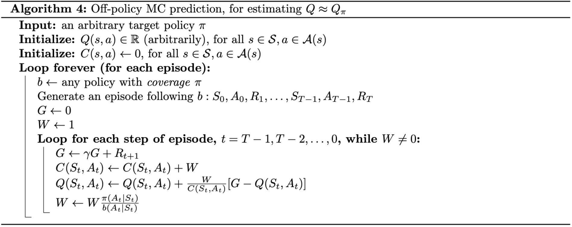
Off-policy Monte Carlo Prediction via Importance Sampling

We apply IS to off-policy learning by weighting returns according to the relative probability of their trajectories occurring under the target and behavior policies, called the importance sampling ratio (which we denoted as $w$ as above, but now we change the notation to $\rho$ in order to follows the book).

The probability of the subsequent state-action trajectory, $A_t,S_{t+1},A_{t+1},\dots,S_T$, occurring under any policy $\pi$ given starting state $s$ is: \begin{align} Pr(A_t,S_{t+1},\dots,S_T|S_t,A_{t:T-1}\sim\pi)&=\pi(A_t|S_t)p(S_{t+1}|S_t,A_t)\dots p(S_T|S_{T-1},A_{T-1}) \\ &=\prod_{k=t}^{T-1}\pi(A_k|S_k)p(S_{k+1}|S_k,A_k) \end{align} Thus, the importance sampling ratio as we defined is: \begin{equation} \rho_{t:T-1}\doteq\dfrac{\prod_{k=t}^{T-1}\pi(A_k|S_k)p(S_{k+1}|S_t,A_t)}{\prod_{k=t}^{T-1}b(A_k|S_k)p(S_{k+1}|S_t,A_t)}=\prod_{k=1}^{T-1}\dfrac{\pi(A_k|S_k)}{b(A_k|S_k)} \end{equation} which depends only on the two policies and the sequence, not on the MDP.

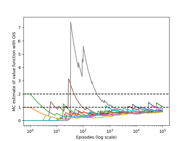
Since $v_b(s)=\mathbb{E}\left[G_t|S_t=s\right]$, then we have \begin{equation} \mathbb{E}\left[\rho_{t:T-1}G_t|S_t=s\right]=v_\pi(s) \end{equation} To estimate $v_\pi(s)$, we simply scale the returns by the ratios and average the results: \begin{equation} V(s)\doteq\dfrac{\sum_{t\in\mathcal{T}(s)}\rho_{t:T(t)-1}G_t}{\vert\mathcal{T}(s)\vert},\tag{5}\label{5} \end{equation} where $\mathcal{T}(s)$ is the set of all states in which $s$ is visited (only for every-visit). For a first-visit,$\mathcal{T}(s)$ would only include time steps that were first visits to $s$ within their episodes. $T(t)$ denotes the first time of termination following time $t$, and $G_t$ denotes the return after $t$ up through $T(t)$.

When importance sampling is done as simple average in this way, we call it ordinary importance sampling (OIS) (which corresponds to unweighted importance sampling in the previous section).

And the one corresponding to weighted importance sampling (WIS), which uses a weighted average, is defined as: \begin{equation} V(s)\doteq\dfrac{\sum_{t\in\mathcal{T}(s)}\rho_{t:T(t)-1}G_t}{\sum_{t\in\mathcal{T}(s)}\rho_{t:T(t)-1}},\tag{6}\label{6} \end{equation} or zero if the denominator is zero.

Incremental Implementation for Off-policy MC Prediction using IS

Incremental Method

Incremental method is a way of updating averages with small, constant computation required to process each new reward instead of maintaining a record of all the rewards and then performing this computation whenever the estimated value was needed. It follows the general rule: \begin{equation} NewEstimate\leftarrow OldEstimate+StepSize\left[Target-OldEstimate\right] \end{equation}

Applying to Off-policy MC Prediction using IS

In ordinary IS, the returns are scaled by the IS ratio $\rho_{t:T(t)-1}$, then simply averaged, as in \eqref{5}. Thus, it’s easy to apply incremental method to OIS.

For WIS, as in the equation \eqref{6}, we have to form a weighted average of the returns, and a slightly different incremental incremental algorithm is required. Suppose we have a sequence of returns $G_1,G_2,\dots,G_{n-1}$, all starting in the same state and each with a corresponding random weight $W_i$, e.g. $W_i=\rho_{t_i:T(t_i)}$. We wish to form the estimate \begin{equation} V_n\doteq\dfrac{\sum_{k=1}^{n-1}W_kG_k}{\sum_{k=1}^{n-1}W_k},\hspace{1cm}n\geq2 \end{equation} and keep it up-to-date as we obtain a single additional return $G_n$. In addition to keeping track of $V_n$, we must maintain for each state the cumulative sum $C_n$ of the weights given to the first $n$ returns. The update rule for $V_n$ is \begin{equation} V_{n+1}\doteq V_n+\dfrac{W_n}{C_n}\big[G_n-V_n\big],\hspace{1cm}n\geq1, \end{equation} and \begin{equation} C_{n+1}\doteq C_n+W_{n+1}, \end{equation} where $C_0=0$. And here is pseudocode of our algorithm.

Off-policy Monte Carlo Control

Similarly, we develop the algorithm for off-policy MC control, based on GPI and WIS, for estimating $\pi_*$ and $q_*$, which is shown below.

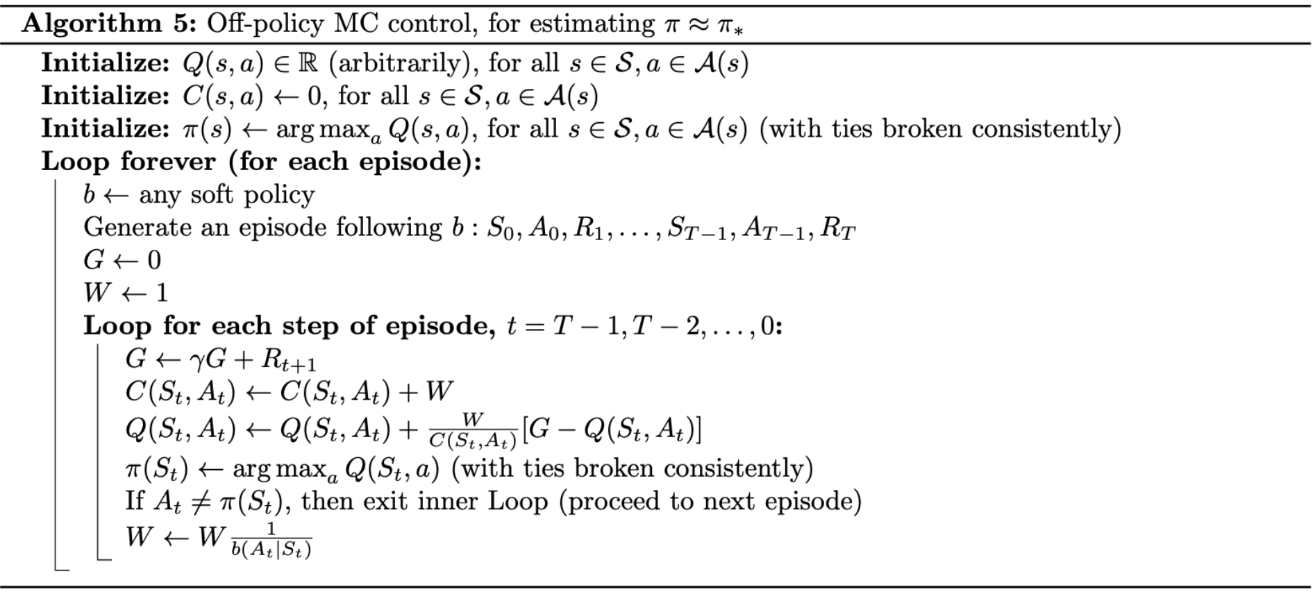
The target policy $\pi\approx\pi_*$ is the greedy policy w.r.t $Q$, which is an estimate of $q_\pi$. The behavior policy, $b$, can be anything, but in order to assure convergence of $\pi$ to the optimal policy, an infinite number of returns must be obtained for each pair of state and action. This can be guaranteed by choosing $b$ to be $\varepsilon$-soft.

The policy $\pi$ converges to optimal at all encountered states even though actions are selected according to a different soft policy $b$, which may change between or even within episodes.

Example - Racetrack

(This example is taken from RL book, Exercise 5.12.)

Problem
Consider driving a race car around a turn like that shown in Figure 4. You want to go as fast as possible, but not so fast as to run off the track. In our simplified racetrack, the car is at one of a discrete set of grid positions, the cells in the diagram. The velocity is also discrete, a number of grid cells moved horizontally and vertically per time step. The actions are increments to the velocity components. Each may be changed by +1, -1, or 0 in each step, for a total of nine (3 x 3) actions. Both velocity components are restricted to be nonnegative and less than 5, and they cannot both be zero except at the starting line. Each episode begins in one of the randomly selected start states with both velocity components zero and ends when the car crosses the finish line. The rewards are -1 for each step until the car crosses the finish line. If the car hits the track boundary, it is moved back to a random position on the starting line, both velocity components are reduced to zero, and the episode continues. Before updating the car’s location at each time step, check to see if the projected path of the car intersects the track boundary. If it intersects the finish line, the episode ends; if it intersects anywhere else, the car is considered to have hit the track boundary and is sent back to the starting line. To make the task more challenging, with probability 0.1 at each time step the velocity increments are both zero, independently of the intended increments. Apply a Monte Carlo control method to this task to compute the optimal policy from each starting state. Exhibit several trajectories following the optimal policy (but turn the noise off for these trajectories).

Solution code (source code can be found here).

We begin by importing some useful packages.

import numpy as np
import matplotlib.pyplot as plt
from tqdm import tqdm

Next, we define our environment

class RaceTrack:

	def __init__(self, grid):
		self.NOISE = 0
		self.MAX_VELOCITY = 4
		self.MIN_VELOCITY = 0
		self.starting_line = []
		self.track = None
		self.car_position = None
		self.actions = [[-1,-1],[-1,0],[-1,1],[0,-1],[0,0],[0,1],[1,-1],[1,0],[1,1]]
		self._load_track(grid)
		self._generate_start_state()
		self.velocity = np.array([0, 0], dtype=np.int16)


	def reset(self):
		self._generate_start_state()
		self.velocity = np.array([0, 0], dtype=np.int16)


	def get_state(self):
		return self.car_position.copy(), self.velocity.copy()


	def _generate_start_state(self):
		index = np.random.choice(len(self.starting_line))
		self.car_position = np.array(self.starting_line[index])


	def take_action(self, action):
		if self.is_terminal():
			return 0
		self._update_state(action)
		return -1


	def _update_state(self, action):
		# update velocity
		# with probability of 0.1, keep the velocity unchanged
		if not np.random.binomial(1, 0.1):
			self.velocity += np.array(action, dtype=np.int16)
			self.velocity = np.minimum(self.velocity, self.MAX_VELOCITY)
			self.velocity = np.maximum(self.velocity, self.MIN_VELOCITY)

		# update car position
		for tstep in range(0, self.MAX_VELOCITY + 1):
			t = tstep / self.MAX_VELOCITY
			position = self.car_position + np.round(self.velocity * t).astype(np.int16)

			if self.track[position[0], position[1]] == -1:
				self.reset()
				return
			if self.track[position[0], position[1]] == 2:
				self.car_position = position
				self.velocity = np.array([0, 0], dtype=np.int16)
				return
		self.car_position = position


	def _load_track(self, grid):
		y_len, x_len = len(grid), len(grid[0])
		self.track = np.zeros((x_len, y_len), dtype=np.int16)
		for y in range(y_len):
			for x in range(x_len):
				pt = grid[y][x]
				if pt == 'W':
					self.track[x, y] = -1
				elif pt == 'o':
					self.track[x, y] = 1
				elif pt == '-':
					self.track[x, y] = 0
				else:
					self.track[x, y] = 2
		# rotate the track in order to sync the track with actions
		self.track = np.fliplr(self.track)
		for y in range(y_len):
			for x in range(x_len):
				if self.track[x, y] == 0:
					self.starting_line.append((x, y))

	def is_terminal(self):
		return self.track[self.car_position[0], self.car_position[1]] == 2

We continue by defining our behavior policy and algorithm.

def behavior_policy(track, state):
	index = np.random.choice(len(track.actions))
	return np.array(track.actions[index])


def off_policy_MC_control(episodes, gamma, grid):
	x_len, y_len = len(grid[0]), len(grid)
	Q = np.zeros((x_len, y_len, 5, 5, 3, 3)) - 40
	C = np.zeros((x_len, y_len, 5, 5, 3, 3))
	pi = np.zeros((x_len, y_len, 5, 5, 1, 2), dtype=np.int16)
	track = RaceTrack(grid)
	# for epsilon-soft greedy policy
	epsilon = 0.1

	for ep in tqdm(range(episodes)):
		track.reset()
		trajectory = []
		while not track.is_terminal():
			state = track.get_state()
			s_x, s_y = state[0][0], state[0][1]
			s_vx, s_vy = state[1][0], state[1][1]
			if not np.random.binomial(1, epsilon):
				action = pi[s_x, s_y, s_vx, s_vy, 0]
			else:
				action = behavior_policy(track, state)
			reward = track.take_action(action)
			trajectory.append([state, action, reward])
		G = 0
		W = 1
		while len(trajectory) > 0:
			state, action, reward = trajectory.pop()
			G = gamma * G + reward
			sp_x, sp_y, sv_x, sv_y = state[0][0], state[0][1], state[1][0], state[1][1]
			a_x, a_y = action
			s_a = (sp_x, sp_y, sv_x, sv_y, a_x, a_y)
			C[s_a] += W
			Q[s_a] += W/C[s_a]*(G-Q[s_a])
			q_max = -1e5
			a_max = None
			for act in track.actions:
				sa_max = sp_x, sp_y, sv_x, sv_y, act[0], act[1]
				if Q[sa_max] > q_max:
					q_max = Q[sa_max]
					a_max = act
			pi[sp_x, sp_y, sv_x, sv_y, 0] = a_max
			if not np.array_equal(pi[sp_x, sp_y, sv_x, sv_y, 0], action):
				break
			W *= 1/(1-epsilon+epsilon/9)
	return pi

And wrapping everything up with the main function.

if __name__ == '__main__':
	gamma = 0.9
	episodes = 10000
	grid = ['WWWWWWWWWWWWWWWWWW',
          'WWWWooooooooooooo+',
          'WWWoooooooooooooo+',
          'WWWoooooooooooooo+',
          'WWooooooooooooooo+',
          'Woooooooooooooooo+',
          'Woooooooooooooooo+',
          'WooooooooooWWWWWWW',
          'WoooooooooWWWWWWWW',
          'WoooooooooWWWWWWWW',
          'WoooooooooWWWWWWWW',
          'WoooooooooWWWWWWWW',
          'WoooooooooWWWWWWWW',
          'WoooooooooWWWWWWWW',
          'WoooooooooWWWWWWWW',
          'WWooooooooWWWWWWWW',
          'WWooooooooWWWWWWWW',
          'WWooooooooWWWWWWWW',
          'WWooooooooWWWWWWWW',
          'WWooooooooWWWWWWWW',
          'WWooooooooWWWWWWWW',
          'WWooooooooWWWWWWWW',
          'WWooooooooWWWWWWWW',
          'WWWoooooooWWWWWWWW',
          'WWWoooooooWWWWWWWW',
          'WWWoooooooWWWWWWWW',
          'WWWoooooooWWWWWWWW',
          'WWWoooooooWWWWWWWW',
          'WWWoooooooWWWWWWWW',
          'WWWoooooooWWWWWWWW',
          'WWWWooooooWWWWWWWW',
          'WWWWooooooWWWWWWWW',
          'WWWW------WWWWWWWW']
	policy = off_policy_MC_control(episodes, gamma, grid)
	track_ = RaceTrack(grid)
	x_len, y_len = len(grid[0]), len(grid)
	trace = np.zeros((x_len, y_len))
	for _ in range(1000):
		state = track_.get_state()
		sp_x, sp_y, sv_x, sv_y = state[0][0], state[0][1], state[1][0], state[1][1]
		trace[sp_x, sp_y] += 1
		action = policy[sp_x, sp_y, sv_x, sv_y, 0]
		reward = track_.take_action(action)
		if track_.is_terminal():
			break
	trace = (trace > 0).astype(np.float32)
	trace += track_.track
	plt.imshow(np.flipud(trace.T))
	plt.savefig('./racetrack_off_policy_control.png')
	plt.close()

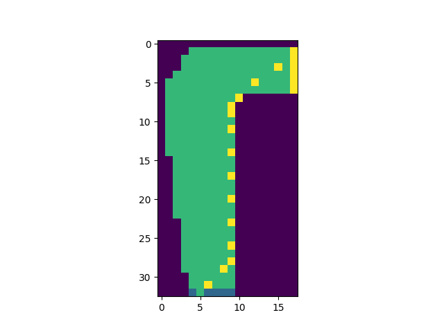
We end up with this result after running the code.

Discounting-aware Importance Sampling

Recall that in the above section, we defined the estimator for $\mathbb{E}_P[f]$ as: \begin{equation} \hat{\mathbb{E}}_\mathcal{D}(f)=\dfrac{1}{M}\sum_{m=1}^{M}f(x[m])\dfrac{P(x[m])}{Q(x[m])} \end{equation} This estimator is unbiased because each of the samples it averages is unbiased: \begin{equation} \mathbb{E}_{Q}\left[\dfrac{P(x[m])}{Q(x[m])}f(x[m])\right]=\int_x Q(x)\dfrac{P(x)}{Q(x)}f(x)\hspace{0.1cm}dx=\int_x P(x)f(x)\hspace{0.1cm}dx=\mathbb{E}_{P}\left[f(x[m])\right] \end{equation} This IS estimate is unfortunately often of unnecessarily high variance. To be more specific, for example, the episodes last 100 steps and $\gamma=0$. Then $G_0=R_1$ will be weighted by \begin{equation} \rho_{0:99}=\dfrac{\pi(A_0|S_0)}{b(A_0|S_0)}\dots\dfrac{\pi(A_{99}|S_{99})}{b(A_{99}|S_{99})} \end{equation} but actually, it really needs to be weighted by $\rho_{0:1}=\frac{\pi(A_0|S_0)}{b(A_0|S_0)}$. The other 99 factors $\frac{\pi(A_1|S_1)}{b(A_1|S_1)}\dots\frac{\pi(A_{99}|S_{99})}{b(A_{99}|S_{99})}$ are irrelevant because after the first reward, the return has already been determined. These later factors are all independent of the return and of expected value $1$; they do not change the expected update, but they add enormously to its variance. They could even make the variance infinite in some cases.

One of the methods used to avoid this large extraneous variance is discounting-aware IS. The idea is to think of discounting as determining a probability of termination or, equivalently, a degree of partial termination.

We begin by defining flat partial returns: \begin{equation} \bar{G}_{t:h}\doteq R_{t+1}+R_{t+2}+\dots+R_h,\hspace{1cm}0\leq t<h\leq T, \end{equation} where flat denotes the absence of discounting, and partial denotes that these returns do not extend all the way to termination but instead stop at $h$, called the horizon. The conventional full return $G_t$ can be viewed as a sum of flat partial returns: \begin{align} G_t&\doteq R_{t+1}+\gamma R_{t+2}+\gamma^2 R_{t+3}+\dots+\gamma^{T-t-1}R_T \\ &=(1-\gamma)R_{t+1} \\ &\hspace{0.5cm}+(1-\gamma)\gamma(R_{t+1}+R_{t+2}) \\ &\hspace{0.5cm}+(1-\gamma)\gamma^2(R_{t+1}+R_{t+2}+R_{t+3}) \\ &\hspace{0.7cm}\vdots \\ &\hspace{0.5cm}+(1-\gamma)\gamma^{T-t-2}(R_{t+1}+R_{t+2}+\dots+R_{T-1}) \\ &\hspace{0.5cm}+\gamma^{T-t-1}(R_{t+1}+R_{t+2}+\dots+R_T) \\ &=(1-\gamma)\sum_{h=t+1}^{T-1}\left(\gamma^{h-t-1}\bar{G}_{t:h}\right)+\gamma^{T-t-1}\bar{G}_{t:T} \end{align} Now we need to scale the flat partial returns by an IS ratio that is similarly truncated. As $\bar{G}_{t:h}$ only involves rewards up to a horizon $h$, we only need the ratio of the probabilities up to $h$. We define:

• Discounting-aware OIS estimator \begin{equation} V(s)\doteq\dfrac{\sum_{t\in\mathcal{T}(s)}\left[(1-\gamma)\sum_{h=t+1}^{T(t)-1}\left(\gamma^{h-t-1}\rho_{t:h-1}\bar{G}_{t:h}\right)+\gamma^{T(t)-t-1}\rho_{t:T(t)-1}\bar{G}_{t:T(t)}\right]}{\vert\mathcal{T}(s)\vert} \end{equation}
• Discounting-aware WIS estimator \begin{equation} V(s)\doteq\dfrac{\sum_{t\in\mathcal{T}(s)}\left[(1-\gamma)\sum_{h=t+1}^{T(t)-1}\left(\gamma^{h-t-1}\rho_{t:h-1}\bar{G}_{t:h}\right)+\gamma^{T(t)-t-1}\rho_{t:T(t)-1}\bar{G}_{t:T(t)}\right]}{\sum_{t\in\mathcal{T}(s)}\left[(1-\gamma)\sum_{h=t+1}^{T(t)-1}\left(\gamma^{h-t-1}\rho_{t:h-1}\right)+\gamma^{T(t)-t-1}\rho_{t:T(t)-1}\right]} \end{equation}

These two estimators take into account the discount rate $\gamma$ but have no effect if $\gamma=1$.

Per-decision Importance Sampling

There is another way beside discounting-aware that may be able to reduce variance, even if $\gamma=1$.

Recall that in the off-policy estimator \eqref{5} and \eqref{6}, each term of the sum in the numerator is itself a sum: \begin{align} \rho_{t:T-1}G_t&=\rho_{t:T-1}\left(R_{t+1}+\gamma R_{t+2}+\dots+\gamma^{T-t-1}R_T\right) \\ &=\rho_{t:T-1}R_{t+1}+\gamma\rho_{t:T-1}R_{t+2}+\dots+\gamma^{T-t-1}\rho_{t:T-1}R_T\tag{7}\label{7} \end{align} We have that \begin{equation} \rho_{t:T-1}R_{t+k}=\dfrac{\pi(A_t|S_t)}{b(A_t|S_t)}\dots\dfrac{\pi(A_{t+k-1}|S_{t+k-1})}{b(A_{t+k-1}|S_{t+k-1})}\dots\dfrac{\pi(A_{T-1}|S_{T-1})}{b(A_{T-1}|S_{T-1})}R_{t+k} \end{equation} Of all these factors, only the first $k$ factors, $\frac{\pi(A_t|S_t)}{b(A_t|S_t)}\dots\frac{\pi(A_{t+k-1}|S_{t+k-1})}{b(A_{t+k-1}|S_{t+k-1})}$, and the last (the reward $R_{t+k}$) are related. All the others are for event that occurred after the reward. Moreover, we have that \begin{equation} \mathbb{E}\left[\dfrac{\pi(A_i|S_i)}{b(A_i|S_i)}\right]\doteq\sum_a b(a|S_i)\dfrac{\pi(a|S_i)}{b(a|S_i)}=1 \end{equation} Therefore, we obtain \begin{align} \mathbb{E}\Big[\rho_{t:T-1}R_{t+k}\Big]&=\mathbb{E}\left[\dfrac{\pi(A_t|S_t)}{b(A_t|S_t)}\dots\dfrac{\pi(A_{t+k-1}|S_{t+k-1})}{b(A_{t+k-1}|S_{t+k-1})}\right]\mathbb{E}\left[\dfrac{\pi(A_k|S_k)}{b(A_k|S_k)}\right]\dots\mathbb{E}\left[\dfrac{\pi(A_{T-1}|S_{T-1})}{b(A_{T-1}|S_{T-1})}\right] \\ &=\mathbb{E}\Big[\rho_{t:t+k-1}R_{t+k}\Big].1\dots 1 \\ &=\mathbb{E}\Big[\rho_{t:t+k-1}R_{t+k}\Big] \end{align} Plug the result we just got into the expectation of \eqref{7}, we have \begin{align} \mathbb{E}\Big[\rho_{t:T-1}G_t\Big]&=\mathbb{E}\Big[\rho_{t:T-1}R_{t+1}+\gamma\rho_{t:T-1}R_{t+2}+\dots+\gamma^{T-t-1}\rho_{t:T-1}R_T\Big] \\ &=\mathbb{E}\Big[\rho_{t:t}R_{t+1}+\gamma\rho_{t:t+1}R_{t+2}+\dots+\gamma^{T-t-1}\rho_{t:T-1}R_T\Big] \\ &=\mathbb{E}\Big[\tilde{G}_t\Big], \end{align} where $\tilde{G}_t=\rho_{t:T-1}R_{t+1}+\gamma\rho_{t:T-1}R_{t+2}+\dots+\gamma^{T-t-1}\rho_{t:T-1}R_T$.

We call this idea per-decision IS. Hence, we develop per-decision OIS estimator, using $\tilde{G}_t$: \begin{equation} V(s)\doteq\dfrac{\sum_{t\in\mathcal{T}(s)}\tilde{G}_t}{\vert\mathcal{T}(s)\vert} \end{equation}

References

[1] Richard S. Sutton, Andrew G. Barto. Reinforcement Learning: An Introduction. MIT press, 2018.

[2] Adrian Barbu, Song-Chun Zhu. Monte Carlo Methods.

[3] David Silver. UCL course on RL.

[4] Csaba Szepesvári. Algorithms for Reinforcement Learning.

[5] Singh, S.P., Sutton, R.S. Reinforcement learning with replacing eligibility traces. Mach Learn 22, 123–158, 1996.

[6] John N. Tsitsiklis. On the Convergence of Optimistic Policy Iteration. Journal of Machine Learning Research 3 (2002) 59–72.

[7] Yuanlong Chen. On the convergence of optimistic policy iteration for stochastic shortest path problem, arXiv:1808.08763, 2018.

[8] Jun Liu. On the Convergence of Reinforcement Learning with Monte Carlo Exploring Starts. arXiv:2007.10916, 2020.

[9] Daphne Koller & Nir Friedman. Probabilistic Graphical Models: Principles and Techniques.

[10] A. Rupam Mahmood, Hado P. van Hasselt, Richard S. Sutton. Weighted importance sampling for off-policy learning with linear function approximation. Advances in Neural Information Processing Systems 27 (NIPS 2014).

Footnotes