You may have known or heard vaguely about a computer program called AlphaGo - the AI has beaten Lee Sedol - the winner of 18 world Go titles. One of the techniques it used is called self-play against its other instances, with Reinforcement Learning.
What is Reinforcement Learning?
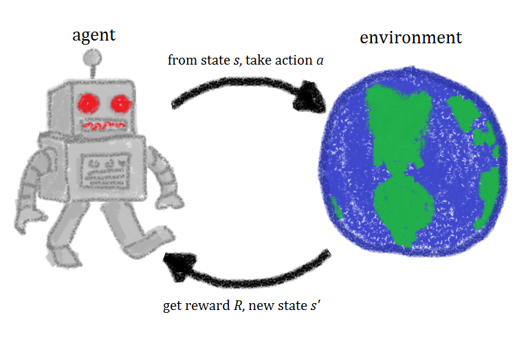
Say, there is an unknown environment that we’re trying to put an agent on. By interacting with the agent through taking actions that gives rise to rewards continually, the agent learns a policy that maximize the cumulative rewards.
Reinforcement Learning (RL), roughly speaking, is an area of Machine Learning that describes methods aimed to learn a good strategy (called policy) for the agent from experimental trials and relative simple feedback received. With the optimal policy, the agent is capable to actively adapt to the environment to maximize future rewards.
Markov Decision Processes (MDPs)
Markov decision processes (MDPs) formally describe an environment for RL. And almost all RL problems can be formalized as MDPs. A Markov decision process is a tuple $⟨\mathcal{S}, \mathcal{A}, \mathcal{P}, \mathcal{R}, \gamma⟩$
- $\mathcal{S}$ is a set of states called state space.
- $\mathcal{A}$ is a set of actions called action space.
- $\mathcal{P}$ is a state transition probability matrix, $\mathcal{P}_{ss’}^a=P(S_{t+1}=s’|S_t=s,A_t=a)$.
- $\mathcal{R}$ is a reward function, $\mathcal{R}_s^a=\mathbb{E}\left[R_{t+1}|S_t=s,A_t=a\right]$.
- $\gamma\in[0, 1]$ is a discount factor for future reward.
MDP is an extension of a Markov chain. If only one action exists for each state, and all rewards are the same, an MDP reduces to a Markov chain. All states in an MDP has Markov property, referring to the fact that the current state captures all relevant information from the history. \begin{equation} P(S_{t+1}|S_t)=P(S_{t+1}|S_1,\dots,S_t) \end{equation}
Return
In the preceding section, we have said that the goal of agent is to maximize the cumulative reward in the long run. In general, we seek to maximize the expected return.
The return $G_t$ is defined to be the total discounted reward from $t$. \begin{equation} G_t=R_{t+1}+\gamma R_{t+2}+\gamma^2 R_{t+3}+\dots=\sum_{k=0}^{\infty}\gamma^k R_{t+k+1}, \end{equation} where $\gamma\in[0,1]$ is called discount rate (or discount factor).
The discount rate $\gamma$ determines the present value of future rewards: a reward received k time steps in the future is worth only $\gamma^{k-1}$ times what it would be worth if it were received immediately. And also, it provides mathematical convenience since as $k\rightarrow\infty$ then $\gamma^k\rightarrow 0$.
Policy
Policy, which is denoted as $\pi$, is the behavior function of the agent. $\pi$ is a mapping from states to probabilities of selecting each possible action. In other words, it lets us know which action to take in the current state $s$ and can be in either deterministic or stochastic form.
- Deterministic policy: $\pi(s)=a$
- Stochastic policy: $\pi(a|s)=P(A_t=a|S_t=s)$
Value Function
Value function measures how good a particular state is (or how good it is to perform a given action in a given state).
The state-value function of a state $s$ under a policy $\pi$, denoted as $v_\pi(s)$, is the expected return starting from state $s$ and following $\pi$ thereafter. \begin{equation} v_\pi(s)=\mathbb{E}_\pi[G_t|S_t=s] \end{equation} Similarly, we define the value of taking action $a$ in state $s$ under a policy $\pi$, denoted as $q_\pi(s,a)$, as the expected return starting from $s$, taking the action $a$, and thereafter following policy $\pi$. \begin{equation} q_\pi(s,a)=\mathbb{E}_\pi[G_t|S_t=s,A_t=a] \end{equation} Since we follow the policy $\pi$, we have that \begin{equation} v_\pi(s)=\sum_{a\in\mathcal{A}}q_\pi(s,a)\pi(a|s) \end{equation}
Optimal Policy and Optimal Value Function
For finite MDPs (finite state and action space), we can precisely define an optimal policy. Value functions define a partial ordering over policies. A policy $\pi$ is defined to be better than or equal to a policy $\pi’$ if its expected return is greater than or equal to that of $\pi’$ for all states. In other words, \begin{equation} \pi\geq\pi’\iff v_\pi(s)\geq v_{\pi’} \forall s\in\mathcal{S} \end{equation}
Theorem 1 (Optimal policy) For any MDP, there exists an optimal policy $\pi_*$ that is better than or equal to all other policies \begin{equation} \pi_*\geq\pi,\forall\pi \end{equation}
Proof
Proof of the above theorem is provided in another note since we need some additional tools to do that.
There may be more than one optimal policy, they share the same state-value function, called optimal state-value function though. \begin{equation} v_*(s)=\max_{\pi}v_\pi(s) \end{equation} Optimal policies also share the same action-value function, called optimal action-value function \begin{equation} q_*(s,a)=\max_{\pi}q_\pi(s,a) \end{equation}
Bellman Equations
A fundamental property of value functions used throughout RL is that they satisfy recursive relationships \begin{align} v_\pi(s)&\doteq \mathbb{E}_\pi[G_t|S_t=s] \\&=\mathbb{E}_\pi[R_t+\gamma G_{t+1}|S_t=s] \\&=\sum_{s’,r,g’,a}p(s’,r,g’,a|s)(r+\gamma g’) \\&=\sum_{a}p(a|s)\sum_{s’,r,g’}p(s’,r,g’|a,s)(r+\gamma g’) \\&=\sum_{a}\pi(a|s)\sum_{s’,r,g’}p(s’,r|a,s)p(g’|s’,r,a,s)(r+\gamma g’) \\&=\sum_{a}\pi(a|s)\sum_{s’,r}p(s’,r|a,s)\sum_{g’}p(g’|s’)(r+\gamma g’) \\&=\sum_{a}\pi(a|s)\sum_{s’,r}p(s’,r|a,s)\left[r+\gamma\sum_{g’}p(g’|s’)g’\right] \\&=\sum_{a}\pi(a|s)\sum_{s’,r}p(s’,r|a,s)\left[r+\gamma v_\pi(s’)\right], \end{align} where $p(s’,r|s,a)=P(S_{t+1}=s’,R_{t+1}=r|S_t=s,A_t=a)$, which defines the dynamics of the MDP. The last equation is called the Bellman equation for $v_\pi(s)$. It expresses a relationship between the value state $s$, $v_\pi(s)$ and the values of its successor states $s’$, $v_\pi(s’)$.
Similarly, we define the Bellman equation for $q_\pi(s,a)$. \begin{align} q_\pi(s,a)&\doteq\mathbb{E}_\pi[G_t|S_t=s,A_t=a] \\&=\mathbb{E}_\pi[R_t+\gamma G_{t+1}|S_t=s,A_t=a] \\&=\sum_{s’,r}p(s’,r|s,a)\left[r+\gamma\sum_{a’}\pi(a’|s’)q_\pi(s’,a’)\right] \end{align}
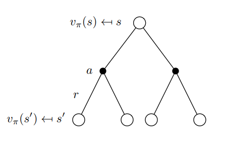
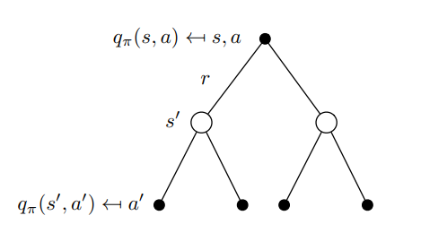
Bellman Backup Diagram
Backup diagram of state-value function and action-value function respectively
Bellman Optimality Equations
Since $v_*$ is the value function for a policy, it must satisfy the Bellman equation for state-values. Moreover, it is also the optimal value function, then we have \begin{align} v_*(s)&=\max_{a\in\mathcal{A(s)}}q_{\pi_*}(s,a) \\&=\max_{a}\mathbb{E}_{\pi_*}[G_t|S_t=s,A_t=a] \\&=\max_{a}\mathbb{E}_{\pi_*}[R_{t+1}+\gamma G_{t+1}|S_t=s,A_t=a] \\&=\max_{a}\mathbb{E}[R_{t+1}+\gamma v_*(S_{t+1})|S_t=s,A_t=a] \\&=\max_{a}\sum_{s’,r}p(s’,r|s,a)[r+\gamma v_*(s’)] \end{align} The last two equations are two forms of the Bellman optimality equation for $v_*$. Similarly, we have the Bellman optimality equation for $q_*$ \begin{align} q_*(s,a)&=\mathbb{E}\left[R_{t+1}+\gamma\max_{a’}q_*(S_{t+1},a’)|S_t=s,A_t=a\right] \\&=\sum_{s’,r}p(s’,r|s,a)\left[r+\gamma\max_{a’}q_*(s’,a’)\right] \end{align}
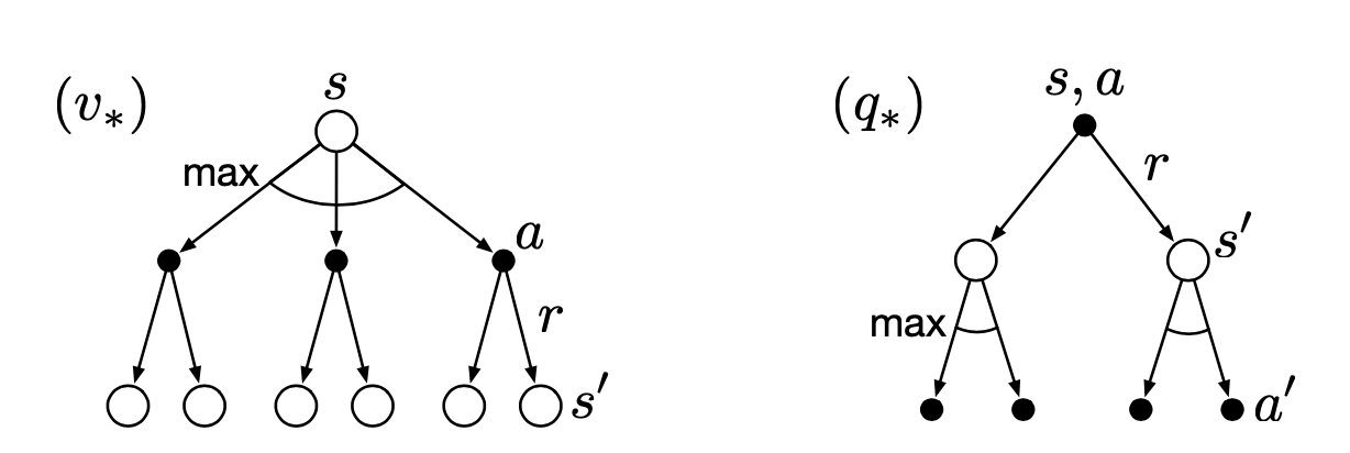
Backup diagram for $v_*$ and $q_*$
References
[1] Richard S. Sutton, Andrew G. Barto. Reinforcement Learning: An Introduction. MIT press, 2018.
[2] David Silver. UCL course on RL.
[3] Lilian Weng A (Long) Peek into Reinforcement Learning. Lil’Log, 2018.
[4] AlphaGo. Deepmind.