Model-based RL with latent variable models

Model-based RL methods that learn latent-variable models instead of trying to predict dynamics models in the observed space. The learned world model then can be used in planning effectively rather than being less efficiently, for instance in visual-based tasks, generating images for future time steps and feed them back into the model to predict the next ones, which requires more computation.

World Models

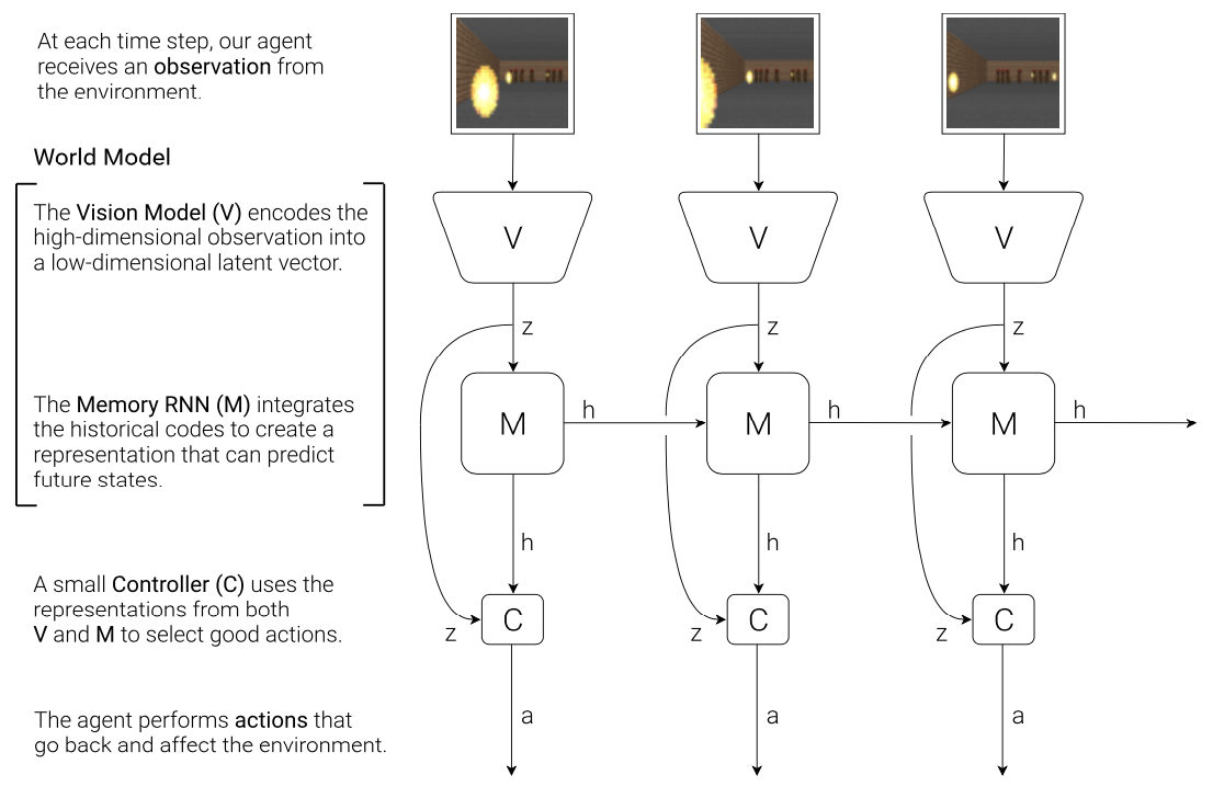
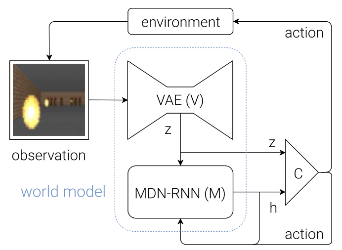
The World Models paper proposed an agent that learns a generative model of the environment such that the model can be used to train a policy entirely in simulation. The agent consists of three components:

• Vision (V) model encodes observations into lower-dimensional representations. It learns an abstract, compressed representation of each input observation at each time step. The paper specifically chose VAE as the V model.
• Memory (M) model predicts future representations based on history. It is an MDN-RNN (an RNN with a Mixture Density Network output layer) served as a predictive model of the future latent vectors $z$ that V is expected to produce. Specifically, the output of M is a probability distribution $p(z)$, which was chosen as a mixture of Gaussian distributions.
• Controller (C) model decides what actions to take based on the representations created by its world model (vision + memory) in order to maximize the cumulative reward of the agent during a rollout. In the paper, C was selected as a single-layer linear model that maps $z_t$ and $h_t$ to action $a_t$ at each time-step: \begin{equation} a_t=W_c\left[\begin{matrix}z_t & h_t\end{matrix}\right]+b_c, \end{equation} where the model is defined by the weight matrix $W_c$ and bias vector $b_c$; and where $\left[\begin{matrix}z_t & h_t\end{matrix}\right]$ is a vector formed by concatenating $z_t$ and $h_t$ together.

Specifically, components are trained separately and the whole algorithm proceeds as:

• Collect rollouts from a random policy.
• Train V model to encode the observations $x$ to latent vectors $z$. Then use the trained model in pre-processing each observation at time-step $t$, $x_t$, into $z_t$.
• Train M to predict $p(z_{t+1}\vert z_t,a_t,h_t)$ where $a_t$ is the action taken at time-step $t$, obtained from rollouts, and $h_t$ is the hidden state of M at time-step $t$.
• Train C using $z_t$ and $h_t$ as inputs. In the original paper, both $z_t$ and $h_t$ are compact representations, and C is a single-layer linear model, which allowed the authors to use CMA-ES as the optimizer for model training.

PlaNet

Deep Planning Network (PlaNet) works in the scope of partially observable Markov decision processes (POMDPs). A partially observable Markov decision process is a tuple of $(\mathcal{S},\mathcal{A},\mathcal{T},R,\Omega ,O,\gamma)$ where:

• $(\mathcal{S},\mathcal{A},\mathcal{T},R,\gamma)$ describes a Markov decision process;
• $\Omega$ is a finite set of observations;
• $O:\mathcal{S}\times\mathcal{A}\to\Pi(\Omega)$ is the observation function, which gives, for each action and resulting state, a probability over possible observations, i.e. $O(s’,a,o)=P(o\mid s’,a)$.

We consider a discrete-time POMDP. At each time-step $t$, we have a state $s_t$, an image observation $o_t$, a continuous action vector $a_t$, and a scalar reward $r_t$ following the stochastic dynamics, which consists of four components

• Transition function: $s_t\sim\text{p}(s_t\mid s_{t-1},a_{t-1})$;
• Observation function: $o_t\sim\text{p}(o_t\mid s_t)$;
• Reward function: $r_t\sim\text{p}(r_t\mid s_t)$;
• Policy: $a_t\sim\text{p}(a_t\mid o_{\leq t},a_{\lt t})$

where we assume a fixed initial state $s_0$ without loss of generality. Our goal is to find a policy $\text{p}(a_t\mid o_{\leq t},a_{<t})$ that maximizes the expected sum of rewards $\mathbb{E}_\text{p}\left[\sum_{t=1}^{H}r_t\right]$ taken over the distributions of the environment and the policy.

Recurrent state-space model

A state-space model (SSM) is a partially observed Markov model where the hidden state, $z_t$, evolves over time to a Markov process, and each hidden state generates some observations $x_t$ at each time-step. The goal is to infer the hidden states given the observations.

An SSM can be represented as a stochastic (discrete-time) nonlinear dynamical system: \begin{align} z_t&=f(z_{t-1},u_t,q_t)\nonumber \\ x_t&=h(z_t,u_t,x_{1:t-1},r_t)\nonumber, \end{align} where $z_t\in\mathbb{R}^{N_z}$ are the hidden states, $u_t\in\mathbb{R}^{N_u}$ are optional observed inputs, $x_t\in\mathbb{R}^{N_x}$ are observed outputs, $f$ is the transition function, $q_t$ is the process noise, $h$ is the observation function, and $r_t$ is the observation noise.

The system can be written as a probabilistic model rather than a deterministic function of random noises: \begin{align} p(z_t\mid z_{t-1},u_t)&=p(z_t\mid f(z_{t-1},u_t))\label{eq:rssm.1} \\ p(x_t\mid z_t,u_t,x_{1:t-1})&=p(x_t\mid h(z_t,u_t,x_{1:t-1}))\label{eq:rssm.2}, \end{align} where $p(z_t\vert z_{t-1},u_t)$ is called the transition (dynamics) model and $p(x_t\vert z_t,u_t,x_{1:t-1})$ is referred as the observation model. Unrolling over time gives us the joint distribution: \begin{equation} p(x_{1:T},z_{1:T}\vert u_{1:T})=p(z_1\vert u_1)\prod_{t=2}^{T}p(z_t\vert z_{t-1},u_t)\prod_{t=1}^{T}p(x_t\vert z_t,u_t,x_{1:t-1})\label{eq:rssm.3} \end{equation} When the observations are assumed to be conditionally independent of each other (rather than having Markov property) given the hidden state, i.e. $x_1\perp\ldots\perp x_T\vert z_t$, the joint distribution \eqref{eq:rssm.3} simplifies into: \begin{equation} p(x_{1:T},z_{1:T}\vert u_{1:T})=p(z_1\vert u_1)\prod_{t=2}^{T}p(z_t\vert z_{t-1},u_t)\prod_{t=1}^{T}p(x_t\vert z_t,u_t)\label{eq:rssm.4} \end{equation} And if there are no observed inputs, as illustrated in Figure 3, \eqref{eq:rssm.4} will further simplify into an unconditional generative model¹: \begin{equation} p(x_{1:T},z_{1:T})=p(z_1)\prod_{t=2}^{T}p(z_t\vert z_{t-1})\prod_{t=1}^{T}p(x_t\vert z_t) \end{equation} If we use neural networks to represent the dynamics model $p(z_t\vert z_{t-1})$ and/or the observation model $p(x_t\vert z_t)$, we end up with the so-called deep Markov model (DMM).

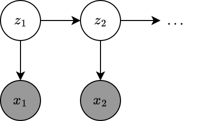
To fit a DMM using variational inference, we first consider the posterior: \begin{align} p(\mathbf{z}\vert\mathbf{x})=p(z_{1:T}\vert x_{1:T})&=p(z_1\vert x_{1:T})\prod_{t=2}^{T}p(z_t\vert z_{t-1},x_{1:T}) \\ &=p(z_1\vert x_{1:T})\prod_{t=2}^{T}p(z_t\vert z_{t-1},x_{1:t-1},x_{t:T}) \\ &=p(z_1\vert x_{1:T})\prod_{t=2}^{T}p(z_t\vert z_{t-1},x_{t:T}), \end{align} where in the last step, we use the fact that $z_t\perp x_{1:t-1}\vert z_{t-1}$, which can be observed directly from Figure 3.

Since the integral of the marginal likelihood is usually intractable, which prevents us from computing the posterior efficiently, we instead approximate $p(z_{1:T}\vert x_{1:T})$ with an inference network.

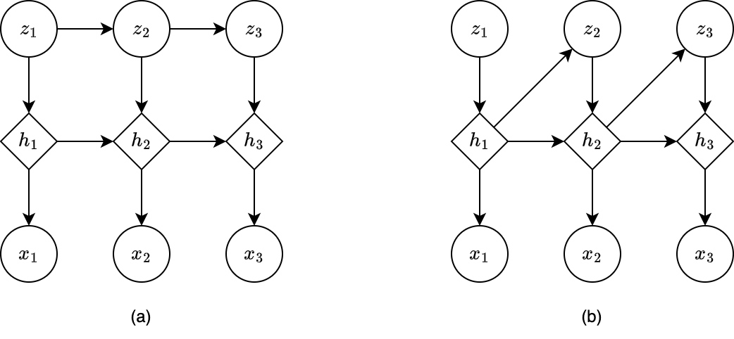
In DMM, the observation model $p(x_t\vert z_t)$ is first-order Markov, as is the dynamics model $p(z_t\vert z_{t-1})$. In order to make the models capture the long-range dependencies, we append deterministic hidden states into the models. Specifically,

• We can make the observation model $p(x_t\vert z_t)$ depend on $z_{1:t}$ rather than $z_t$ only by using $p(x_t\vert h_t)$, where $h_t=f(h_{t-1},z_t)$, which allows $h_t$ to record all the stochastic choices, as illustrated in Figure 4a.
• We can also make the dynamics model $p(z_t\vert z_{t-1})$ depend on $z_{1:t-1}$ instead of just $z_{t-1}$ by using $p(z_t\vert h_{t-1})$, as illustrated in Figure 4b.

This is known as a recurrent state-space model (RSSM).

World model

PlaNet uses a SSM as the world model for planning, as illustrated in Figure 5a, which consists of²:

• Transition model: $s_t\sim p(s_t\mid s_{t-1},a_{t-1})$, a Gaussian with mean and variance parameterized by a feed-forward network.
• Observation model: $o_t\sim p(o_t\mid s_t)$, a Gaussian with mean parameterized by a deconvolutional network and identity covariance
• Reward model: $r_t\sim p(r_t\mid s_t)$, a scalar Gaussian with mean parameterized by a feed-forward network and unit variance.

where we assume a fixed initial state $s_0$ without loss of generality.

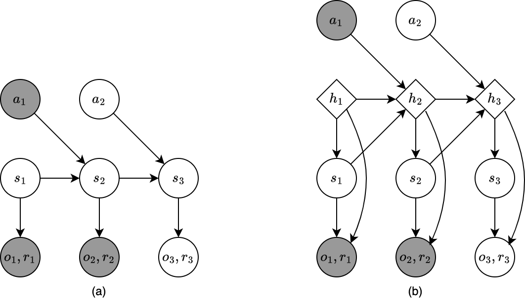
Let us consider the latent dynamics for predicting the observations only, i.e. $p(o_{1:T},s_{1:T}\vert a_{1:T})=\prod_{t=1}^{T}p(s_t\vert s_{t-1},a_{t-1})p(o_t\vert s_t)$, the one for predicting rewards follows by analogy. Since the model is non-linear, the posterior, $p(s_{1:T}\vert o_{1:T},a_{1:T})$ is then intractable. We instead have to use a recognition model (encoder), $q(s_{1:T}\vert o_{1:T},a_{1:T})$, to approximate the state posteriors from past observations and actions: \begin{equation} p(s_{1:T}\vert o_{1:T},a_{1:T})\approx q(s_{1:T}\vert o_{1:T},a_{1:T})=\prod_{t=1}^{T}q(s_t\vert s_{t-1},a_{t-1},o_t)=\prod_{t=1}^{T}q(s_t\vert o_{\leq t},a_{\lt t}), \end{equation} where $q(s_t\vert s_{t-1},a_{t-1},o_t)$ is a diagonal Gaussian with mean and variance parameterized by a CNN followed by an MLP. The variational lower bound (ELBO) corresponding to this encoder is then given as: \begin{align} &\hspace{-1cm}\log p(o_{1:T}\vert a_{1:T})\nonumber \\ &\doteq\log\int\prod_{t=1}^{T}p(s_t\vert s_{t-1},a_{t-1})p(o_t\vert s_t)d s_{1:T} \\ &=\log\mathbb{E}_{p(s_{1:T}\vert a_{1:T})}\left[\prod_{t=1}^{T}p(o_t\vert s_t)\right] \\ &=\log\mathbb{E}_{q(s_{1:T}\vert o_{1:T},a_{1:T})}\left[\prod_{t=1}^{T}p(o_t\vert s_t)\frac{p(s_t\vert s_{t-1},a_{t-1})}{q(s_t\vert o_{\leq t},a_{\lt t})}\right] \\ &\geq\mathbb{E}_{q(s_{1:T}\vert o_{1:T},a_{1:T})}\left[\log\prod_{t=1}^{T}p(o_t\vert s_t)\frac{p(s_t\vert s_{t-1},a_{t-1})}{q(s_t\vert o_{\leq t},a_{\lt t})}\right] \\ &=\mathbb{E}_{q(s_{1:T}\vert o_{1:T},a_{1:T})}\left[\sum_{t=1}^{T}\log p(o_t\vert s_t)+\log p(s_t\vert s_{t-1},a_{t-1})-\log q(s_t\vert o_{\leq t},a_{\lt t})\right] \\ &=\sum_{t=1}^{T}\left(\mathbb{E}_{q(s_t\vert o_{\leq t},a_{\lt t})}\Big[\log p(o_t\vert s_t)\Big]\right.\nonumber \\ &\hspace{1cm}\Big.-\mathbb{E}_{q(s_{t-1}\vert o_{\leq t-1},a_{\lt t-1})}\Big[D_\text{KL}\big(q(s_t\vert o_{\leq t},a_{\lt t})\big\Vert p(s_t\vert s_{t-1},a_{t-1})\big)\Big]\Big),\label{eq:pwr.1} \end{align} where we use Jensen’s inequality in the forth step. The first term inside the parentheses, $\mathbb{E}_{q(s_t\vert o\leq t,a\lt t)}\big[\log p(o_t\vert s_t)\big]$, is the reconstruction loss, which is illustrated in Figure 6a as the edge $s_{t\vert t}\to o_t$. The other one, $\mathbb{E}_{q(s_{t-1}\vert o_{\leq t-1},a_{\lt t-1})}\big[D_\text{KL}(q(s_t\vert o_{\leq t},a_{\lt t})\Vert p(s_t\vert s_{t-1},a_{t-1}))\big]$, is the KL-divergence regularizer, corresponds to the edge $s_{t\vert t}\color{blue}{\to}s_{t\vert t-1}$.

As mentioned above, in order to capture information for multiple time-steps, we need to introduce deterministic hidden states to our SSM, which leads to a RSSM, as illustrated in Figure 5b.

Specifically, the authors added long-range dependencies into the transition model by splitting the state into a stochastic part $s_t$ and a deterministic part $h_t$, which depends on the stochastic and deterministic parts at the previous time-step, $s_{t-1}$ and $h_{t-1}$ respectively. The result model is then given as: \begin{equation} \begin{aligned} &\small\text{Deterministic state model}:&&h_t=f(h_{t-1},s_{t-1},a_{t-1}) \\ &\small\text{Stochastic state model}:&&s_t\sim p(s_t\mid h_t) \\ &\small\text{Observation model}:&&o_t\sim p(o_t\mid h_t,s_t) \\ &\small\text{Reward model}:&&r_t\sim p(r_t\mid h_t,s_t), \end{aligned} \end{equation} where $f(h_{t-1},s_{t-1},a_{t-1})$ is a RNN. We also use the encoder $q(s_{1:T}\mid o_{1:T},a_{1:T})=\prod_{t=1}^{T}q(s_t\mid h_t,o_t)$ to parameterize the approximate state posteriors.

Latent overshooting

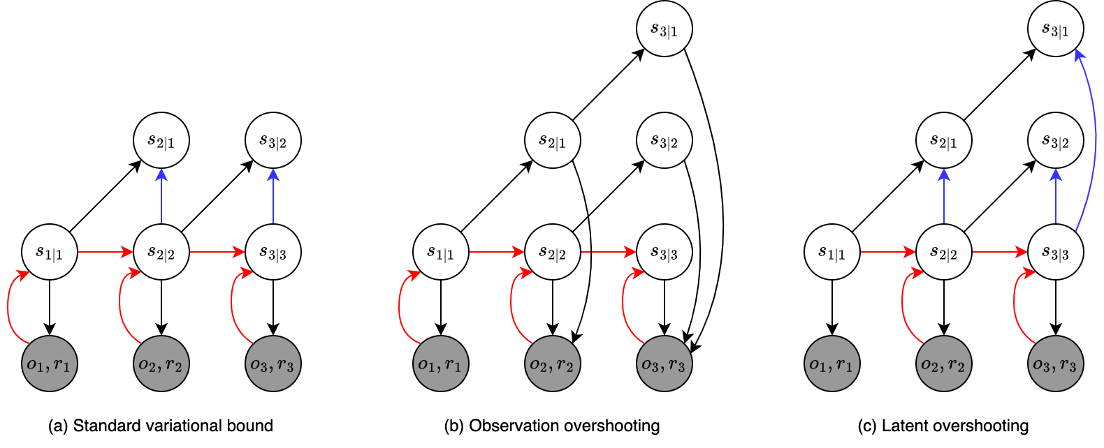
A limitation of using the variational bound given in \eqref{eq:pwr.1} as the objective function is that the stochastic path of the transition function $p(s_t\vert s_{t-1},a_{t-1})$ is only trained through the KL-divergence regularizers for one-step prediction.

One solution to this is to make multi-step forwards predictions using the dynamics model, and use these to reconstruct future observations, and add these errors as extra reconstruction loss terms. This approach is referred as observation overshooting, illustrated in Figure 6b.

Unfortunately, this method is computational expensive, especially in image-based domain. Instead, PlaNet applied the analogous idea but in latent space. To be more specific, let us consider the $d$-step predictive distribution: \begin{equation} p_d(o_{1:T},s_{1:T}\vert a_{1:T})=\prod_{t=1}^{T}p(s_t\vert s_{t-d},a_{t-d-1:t-1})p(o_t\vert s_t), \end{equation} where the multi-step prediction, $p(s_t\vert s_{t-d},a_{t-d-1:t-1})$, is computed by repeatedly applying the transition model, $p(s_\tau\vert s_{\tau-1},a_{\tau-1})$, and integrating out the intermediate states: \begin{align} p(s_t\vert s_{t-d},a_{t-d-1:t-1})&\doteq\int\prod_{\tau=t-d+1}^{t}p(s_\tau\vert s_{\tau-1},a_{\tau-1})d s_{t-d+1:t-1} \\ &=\mathbb{E}_{p(s_{t-1}\vert s_{t-d},a_{t-d-1:t-2})}\big[p(s_t\vert s_{t-1},a_{t-1})\big]\label{eq:lo.1} \end{align} The ELBO corresponding to this $d$-step predictive distribution then can be computed as: \begin{align} &\hspace{-1cm}p_d(o_{1:T}\vert a_{1:T})\nonumber \\ &\doteq\log\int\prod_{t=1}^{T}p(s_t\vert s_{t-d},a_{t-1})p(o_t\vert s_t)d s_{1:T} \\ &=\log\mathbb{E}_{p_d(s_{t:T}\vert a_{1:T})}\left[\prod_{t=1}^{T}p(o_t\vert s_t)\right] \\ &=\log\mathbb{E}_{q(s_{1:T}\vert o_{1:T},a_{1:T})}\left[\prod_{t=1}^{T}p(o_t\vert s_t)\frac{p(s_t\vert s_{t-d},a_{t-d-1:t-1})}{q(s_t\vert o_{\leq t},a_{\lt t})}\right] \\ &\overset{\text{(i)}}{\geq}\mathbb{E}_{q(s_{1:T}\vert o_{1:T},a_{1:T})}\left[\log\prod_{t=1}^{T}p(o_t\vert s_t)\frac{p(s_t\vert s_{t-d},a_{t-d-1:t-1})}{q(s_t\vert o_{\leq t},a_{\lt t})}\right] \\ &=\mathbb{E}_{q(s_{1:T}\vert o_{1:T},a_{1:T})}\left[\sum_{t=1}^{T}\log p(o_t\vert s_t)+\log p(s_t\vert s_{t-d},a_{t-d-1:t-1})-\log q(s_t\vert o_{\leq t},a_{\lt t})\right] \\ &\overset{\text{(ii)}}{=}\mathbb{E}_{q(s_{1:T}\vert o_{1:T},a_{1:T})}\left[\sum_{t=1}^{T}\log p(o_t\vert s_t)+\log\mathbb{E}_{p(s_{t-1}\vert s_{t-d},a_{t-d-1:t-2})}\big[p(s_t\vert s_{t-1},a_{t-1})\big]\right.\nonumber \\ &\hspace{4cm}\Bigg.-\log q(s_t\vert o_{\leq t},a_{\lt t})\Bigg] \\ &\overset{\text{(iii)}}{\geq}\mathbb{E}_{q(s_{1:T}\vert o_{1:T},a_{1:T})}\left[\sum_{t=1}^{T}\log p(o_t\vert s_t)+\mathbb{E}_{p(s_{t-1}\vert s_{t-d},a_{t-d-1:t-2})}\big[\log p(s_t\vert s_{t-1},a_{t-1})\big]\right.\nonumber \\ &\hspace{4cm}\Bigg.-\log q(s_t\vert o_{\leq t},a_{\lt t})\Bigg] \\ &=\sum_{t=1}^{T}\Bigg(\mathbb{E}_{q(s_t\vert o_{\leq t},a_{\lt t})}\big[\log p(o_t\vert s_t)\big]\Bigg.\nonumber \\ &\hspace{1cm}\Bigg.-\mathbb{E}_{p(s_{t-1}\vert s_{t-d},a_{t-d-1:t-2})q(s_{t-d}\vert o_{\leq t-d},a_{\lt t-d})}\Big[D_\text{KL}\big(q(s_t\vert o_{\leq t},a_{\lt t})\big\Vert p(s_t\vert s_{t-1},a_{t-1})\big)\Big]\Bigg), \end{align} where we use Jensen’s inequality for $\log$ function in steps $\text{(i)}$ and $\text{(iii)}$ as well, and step $\text{(ii)}$ comes from equation \eqref{eq:lo.1}.

The above variational bound can be used as the objective function for training the $d$-step predictive distribution. In order to be used for planning, the model instead has to be good at predicting for all distances up to the planning horizon $H$. This gives rise to the latent overshooting, an objective function that generalizes standard variational bound \eqref{eq:pwr.1} for training the model on multi-step predictions of all distances $1\leq d\leq H$, as illustrated in Figure 6c. \begin{align} &\hspace{-1cm}\frac{1}{H}\sum_{d=1}^{H}\log p_d(o_{1:T}\vert a_{1:T})\geq\sum_{t=1}^{T}\Bigg(\mathbb{E}_{q(s_t\vert o_{\leq t},a_{\lt t})}\big[\log p(o_t\vert s_t)\big]\Bigg.\nonumber \\ &\hspace{-0.5cm}\Bigg.-\frac{1}{H}\sum_{d=1}^{H}\beta_d\mathbb{E}_{p(s_{t-1}\vert s_{t-d},a_{t-d-1:t-2})q(s_{t-d}\vert o_{\leq t-d},a_{\lt t-d})}\Big[D_\text{KL}\big(q(s_t\vert o_{\leq t},a_{\lt t})\big\Vert p(s_t\vert s_{t-1},a_{t-1})\big)\Big]\Bigg), \end{align} where $\{\beta_d\}_{d=1}^{H}$ are some hyperparameters as in $\beta$-VAE.

Planning algorithm

PlaNet uses the cross entropy method (CEM) to search for the best action sequence under some current latent dynamics. The method proceeds as:

• Given the current time-step $t$ and the current state belief $q(s_t\vert o_{\leq t},a_{\lt t})$, we define a diagonal Gaussian belief over action sequences \begin{equation} q(a_{t:t+H})\sim\mathcal{N}(\mu_{t:t+H},\sigma_{t:t+H}^2 I), \end{equation} where $H$ is the planning horizon.
• Starting from zero mean, $\mu_{t:t+H}=0$, and unit variance, $\sigma_{t:t+H}^2=1$, repeatedly sample $J$ trajectories and sum the mean rewards predicted along each trajectory: \begin{align} a_{t:t+H}^{(j)}&\sim q(a_{t:t+H}) \\ s_{t:t+H}^{(j)}&\sim q(s_t\vert o_{1:t},a_{1:t-1})\prod_{\tau=t+1}^{t+H+1}p(s_\tau\vert s_{\tau-1},a_{\tau-1}^{(j)}) \\ R^{(j)}&=\sum_{\tau=t+1}^{t+H+1}\mathbb{E}\big[p(r_\tau\vert s_\tau^{(j)})\big] \end{align}
• Evaluate generated trajectories based on their total mean rewards to select $K$ best action sequences: \begin{equation} \mathcal{K}=\text{argsort}(\{R^{(j)}\}_{j=1}^J)_{1:K} \end{equation}
• Refit the belief to the newly obtained top $K$ action sequences \begin{align} \mu_{t:t+H}&=\frac{1}{K}\sum_{k\in\mathcal{K}}a_{t:t+H}^{(k)} \\ \sigma_{t:t+H}&=\frac{1}{K-1}\sum_{k\in\mathcal{K}}\left\vert a_{t:t+H}^{(k)}-\mu_{t:t+H}\right\vert \end{align}
• After some number of iterations of repeatedly performing steps (2) + (3) + (4), the planner returns the first action having mean of the belief for the current time-step, $\mu_t$.

Dreamer

Proposed by the same author of PlaNet, Dreamer improves the computational efficient of its predecessor by replacing the MPC planner by a policy network, which is learned simultaneously with a value network using actor-critic in latent space. Specifically, Dreamer consists of three components, as illustrated in Figure 7, performed in parallel or interleaved:

• Dynamics learning: learning the latent dynamics model from past experience to predict future rewards from actions and past observations.
• Behavior learning: learning action and value models from predicted latent trajectories.
• Environment acting: generating experience by executing the learned action model in the world.

Latent dynamics learning

Analogous to PlaNet, Dreamer also learns a dynamics model via a RSSM. Specifically, recalling for completeness, the world model in Dreamer consists of: \begin{equation} \begin{aligned} &\small\text{Recurrent model}:&&h_t=f_\theta(h_{t-1},s_{t-1},a_{t-1}) \\ &\small\text{Representation model}:&&s_t\sim q_\theta(s_t\vert h_t,o_t) \\ &\small\text{Transition model}:&&\hat{s}_t\sim p_\theta(\hat{s}_t\vert h_t) \\ &\small\text{Observation model}:&&\hat{o}_t\sim p_\theta(\hat{o}_t\vert h_t, s_t) \\ &\small\text{Reward model}:&&\hat{r}_t\sim p_\theta(\hat{r}_t\vert h_t,s_t), \end{aligned} \end{equation} where $f_\theta$ is an RNN and $\theta$ is the joint parameter.

Behavior learning

Since the compact model states $s_t$ are Markovian, the latent dynamics then define an MDP that is fully observed. Letting $\tau$ denote the time index for all quantities in this MDP, each imagined trajectory $\{(s_\tau,a_\tau,r_\tau)\}_{\tau=t}$ starts at a true state, $s_\tau=s_t$ for $\tau=0$ and follow predictions of: \begin{equation} \begin{aligned} &\small\text{Transition model:}&&s_\tau\sim q(s_\tau\vert s_{\tau-1},a_{\tau-1}) \\ &\small\text{Reward model:}&&r_\tau\sim q(r_\tau\vert s_\tau) \\ &\small\text{Policy:}&&a_\tau\sim q(a_\tau\vert s_\tau) \end{aligned} \end{equation} The object is to maximize the expected cumulative imagined rewards $\mathbb{E}_q\left[\sum_{\tau=t}^{\infty}\gamma^{\tau-t}r_\tau\right]$ taken over the policy $q(a_\tau\vert s_\tau)$.

Consider imagined trajectories with a finite horizon $H$. Within the latent space, Dreamer learns an action model (actor) $q_\phi$, parameterized by $\phi$, that aims to predict actions that solve the imagination environment \begin{equation} a_\tau\sim q_\phi(a_\tau\vert s_\tau) \end{equation} At the same time, it also learns a value model (critic) $v_\psi$, parameterized by $\psi$, that estimates the expected cumulative imagined rewards that the action model achieves from each state $s_\tau$ \begin{equation} v_\psi(s_\tau)\approx\mathbb{E}_{q(\cdot\vert s_\tau)}\left[\sum_{\tau=t}^{t+H}\gamma^{\tau-t}r_\tau\right] \end{equation} In the paper, both models are implemented as MLPs. The actor $q_\phi$ outputs a $\tanh$-transformed Gaussian with sufficient statistics predicted by the network, as in SAC. \begin{equation} a_\tau=\tanh(\mu_\phi(s_\tau)+\sigma_\phi(s_\tau)\epsilon),\hspace{1cm}\epsilon\sim\mathcal{N}(0,I) \end{equation} In order to learn the action and value models, we need to estimate the state values of imagined trajectories $\{s_\tau,a_\tau,r_\tau\}_{\tau=t}^{t+H}$, Dreamer, in particular, uses the $\lambda$-return: \begin{align} V_N^k(s_\tau)&\doteq\mathbb{E}_{q_\phi,q_\theta}\left[\sum_{n=\tau}^{h-1}\gamma^{n-\tau}r_n+\gamma^{h-\tau}v_\psi(s_h)\right],\hspace{1cm}h=\min(\tau+k,t+H) \\ V_\lambda(s_\tau)&\doteq(1-\lambda)\sum_{n=1}^{H-1}\lambda^{n-1}V_N^n(s_\tau)+\lambda^{H-1}V_N^H(s_\tau), \end{align} where $V_N^k$ is the $k$-step return, which estimates rewards beyond $k$ steps with the learned value model $v_\psi(s_h)$.

Once the $\lambda$-returns $V_\lambda(s_\tau)$ for all $s_\tau$ along the imagined trajectories are computed, the parameters $\phi$ and $\psi$ can be updated iteratively by SGD according to the actor loss and critic loss respectively: \begin{align} \mathcal{L}_\phi&=-\mathbb{E}_{q_\theta,q_\phi}\left[\sum_{\tau=t}^{t+H}V_\lambda(s_\tau)\right] \\ \mathcal{L}_\psi&=\mathbb{E}_{q_\theta,q_\phi}\left[\sum_{\tau=t}^{t+H}\frac{1}{2}\big\Vert v_\psi(s_\tau)-V_\lambda(s_\tau)\big\Vert_2^2\right] \end{align}

DreamerV2

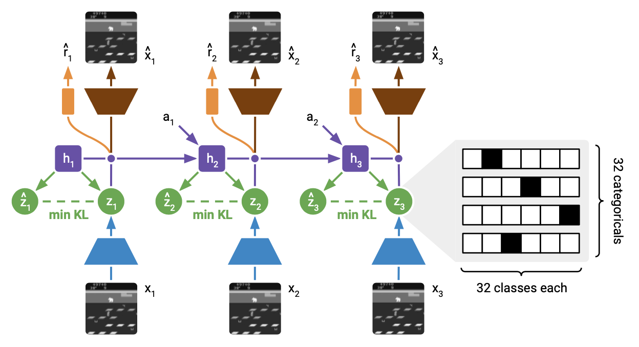
DreamerV2 builds upon the world model introduced in PlaNet and subsequently used by Dreamer, by replacing the Gaussian latent variables with categorical latent variables.

World model learning

Specifically, the world model in DreamerV2, as described in Figure 8, consists of an image encoder (representation model), a RSSM to learn the dynamics and predictors for the image, reward and discount factor.

• Recurrent model: $h_t=f_\theta(h_{t-1},s_{t-1},a_{t-1})$, computes the deterministic recurrent states $h_t$, and $f_\theta$ is a Gated Recurrent Unit (GRU).
• Representation model: $s_t\sim q_\theta(s_t\mid h_t,o_t)$, is a CNN followed by a MLP, and outputs a distribution over posterior stochastic state $s_t$ from the deterministic recurrent state $h_t$ and image $o_t$.
• Transition predictor: $\hat{s}_t\sim p_\theta(\hat{s}_t\mid h_t)$, outputs a distribution over prior stochastic state $\hat{s}_t$ solely from the deterministic recurrent state $h_t$.
• Image predictor: $\hat{o}_t\sim p_\theta(\hat{o}_t\mid h_t,s_t)$, is a transposed CNN (deconvolutional), and outputs a diagonal Gaussian with unit variance.
• Reward predictor: $\hat{r}_t\sim p_\theta(\hat{r}_t\mid h_t,s_t)$, is an MLP, and outputs a univariate Gaussian with unit variance.
• Discount predictor: $\hat{\gamma}_t\sim p_\theta(\hat{\gamma}_t\mid h_t,s_t)$, is an MLP, and outputs a Bernoulli likelihood.

Rather than being a diagonal Gaussian (that used reparameterization trick to compute its gradient) as PlaNet or Dreamer, the stochastic state ($s_t$ and $\hat{s}_t$) in DreamerV2 is a vector of multiple categorical variables that can be optimized using straight-through estimators or Gumbel-Max trick.

All components of the world model are optimized jointly by minimizing the loss function w.r.t $\theta$: \begin{align} \mathcal{L}(\theta)&=\mathbb{E}_{q_\theta(s_{1:T}\vert a_{1:T},o_{1:T})}\left[\sum_{t=1}^{T}\underbrace{-\log p_\theta(o_t\vert h_t,s_t)}_\color{red}{\text{image log loss}}\hspace{0.1cm}\underbrace{-\log p_\theta(r_t\vert h_t,s_t)}_\color{red}{\text{reward log loss}}\hspace{0.1cm}\underbrace{-\log p_\theta(\gamma\vert h_t,s_t)}_\color{red}{\text{discount log loss}}\right.\nonumber \\ &\hspace{4cm}\left.\underbrace{+\beta D_\text{KL}\big[q_\theta(s_t\vert h_t,o_t)\parallel p_\theta(s_t\vert h_t)\big]}_\color{blue}{\text{KL loss}}\right] \end{align} The first three losses act as reconstruction losses for image, reward and discount factor where their corresponding predictors are trained to maximize the log-likelihood of their targets . At the same time, the KL loss acts as a regularizer. Or in other words, the loss function is an ELBO and the world model thus can be interpreted as a sequential VAE where the representation model is an approximate posterior. In order to encourage learning an accurate prior over increasing posterior entropy through minimizing the KL loss so that prior better approximate the aggregate posterior, we split the KL into two parts, with different learning rates. In particular, the loss function changes into: \begin{align} \mathcal{L}(\theta)&=\mathbb{E}_{q_\theta(s_{1:T}\vert a_{1:T},o_{1:T})}\left[\sum_{t=1}^{T}\underbrace{-\log p_\theta(o_t\vert h_t,s_t)}_\text{image log loss}\hspace{0.1cm}\underbrace{-\log p_\theta(r_t\vert h_t,s_t)}_\text{reward log loss}\hspace{0.1cm}\underbrace{-\log p_\theta(\gamma\vert h_t,s_t)}_\text{discount log loss}\right.\nonumber \\ &\hspace{4cm}\left.\underbrace{+\beta(1-\alpha)\log q_\theta(s_t\mid h_t,o_t)}_\text{entropy regularizer}\hspace{0.1cm}\underbrace{-\beta\alpha\log p_\theta(s_t\mid h_t)}_\text{transition loss}\right] \end{align}

Behavior learning

Same as Dreamer, DreamerV2 learns behaviors within its world model using actor-critic method. We first begin by describing the imagination MDP. The MDP can be described as the transition of tuple $(\hat{s}_t,\hat{a}_t,\hat{r}_t,\hat{s}_{t+1})$ over time:

• Starting from $\hat{s}_0$, whose distribution is the distribution of compact model states, i.e. the concatenation of deterministic state and a sample of the stochastic state, the transition predictor $p_\theta(\hat{s}_t\mid\hat{s}_{t-1},\hat{a}_{t-1})$ generates sequences $\hat{s}_{1:H}$ of compact model states up to the imagination horizon $H$.
• The mean of the reward predictor $p_\theta(\hat{r}_t\mid\hat{s}_t)$ is used as imagination reward sequence $\hat{r}_{1:H}$.
• And the discount predictor $p_\theta(\hat{\gamma}_t\mid\hat{s}_t)$ generates the discount sequence $\hat{\gamma}_{1:H}$.

Within the latent space, DreamerV2 learns a stochastic actor and deterministic critic parameterized by $\phi$ and $\psi$ respectively: \begin{equation} \begin{aligned} \hat{a}_t&\sim p_\phi(\hat{a}_t\mid\hat{s}_t) \\ v_\psi(\hat{s}_t)&\approx\mathbb{E}_{p_\theta,p_\phi}\left[\sum_{\tau=t}^{t+H}\hat{\gamma}^{\tau-t}\hat{r}_\tau\right] \end{aligned} \end{equation} The critic is optimized by minimizing the loss function w.r.t $\psi$³: \begin{equation} \mathcal{L}(\psi)=\mathbb{E}_{p_\theta,p_\phi}\left[\sum_{t=1}^{H-1}\frac{1}{2}\big\Vert v_\psi(\hat{s}_t)-\text{sg}(V_t^\lambda)\big\Vert_2^2\right], \end{equation} where to stabilize the training, DreamerV2 utilizes a target network as Deep Q-Learning. In the above equation, $\text{sg}(\cdot)$ denotes the stopping gradient operator and $V_t^\lambda$ is the more general version of $\lambda$-return, defined recursively as: \begin{equation} V_t^\lambda=\hat{r}_t+\hat{\gamma}_t\begin{cases}(1-\lambda)v_\psi(\hat{s}_{t+1})+\lambda V_{t+1}^\lambda &\text{if }t\lt H \\ v_\psi(\hat{s}_H) &\text{if }t=H\end{cases} \end{equation} Analogous to Dreamer, the actor in DreamerV2 is trained to maximize the $\lambda$-return $V_t^\lambda$. But different from its previous version, DreamerV2 also adds REINFORCE gradients using $v_\psi(\hat{s}_t)$ as baseline for variance reduction. This term has learning rate $\rho$ while the straight-through gradients, which backpropagate directly through the learned dynamics, as in Dreamer, goes with learning rate $1-\rho$. It also regularizes the entropy of the actor for exploration purpose. Specifically, the actor is optimized by minimizing the loss function w.r.t $\phi$ \begin{equation} \hspace{-0.5cm}\mathcal{L}(\phi)=\mathbb{E}_{p_\theta,p_\phi}\left[\sum_{t=1}^{H-1}\underbrace{-\rho\log p_\phi(\hat{a}_t\mid\hat{s}_t)\text{sg}(V_t^\lambda-v_\psi(\hat{s}_t))}_\color{orange}{\text{reinforce}}\hspace{0.1cm}\underbrace{-(1-\rho)V_t^\lambda}_{\substack{\color{green}{\text{dynamics}} \\ \color{green}{\text{backprop}}}}\hspace{0.1cm}\underbrace{-\eta H(a_t\vert\hat{s}_t)}_{\substack{\color{purple}{\text{entropy}} \\ \color{purple}{\text{regularizer}}}}\right] \end{equation}

DreamerV3

TD-MPC

Task-oriented latent dynamics model

The dynamics and behaviors in TD-MPC is learned through a Task-Oriented Latent Dynamics (TOLD) model, which comprises five learned components $h_\theta,d_\theta,R_\theta,Q_\theta,\pi_\theta$ that predict the following quantities: \begin{equation} \begin{aligned} &\small\text{Representation}:&&z_t=h_\theta(s_t) \\ &\small\text{Latent dynamics}:&&z_{t+1}=d_\theta(z_t,a_t) \\ &\small\text{Reward}:&&\hat{r}_t=R_\theta(z_t,a_t) \\ &\small\text{Value}:&&\hat{q}_t=Q_\theta(z_t,a_t) \\ &\small\text{Policy}:&&\hat{a}_t\sim\pi_\theta(z_t) \end{aligned} \end{equation} All components of TOLD are trained jointly by minimizing the loss function: \begin{equation} \mathcal{J}(\theta;\Gamma)=\sum_{i=1}^{t+H}\lambda^{i-t}\mathcal{L}(\theta;\Gamma_i), \end{equation} where $\Gamma=(s_t,a_t,r_t,s_{t+1})_{t:t+H}$ is a trajectory sampled from a replay buffer; $\lambda\in\mathbb{R}^+$ is a weighted constant; and $\mathcal{L}(\theta;\Gamma_i)$ is the single-step loss, defined as a combination of three losses: \begin{align} \mathcal{L}(\theta;\Gamma_i)&=c_1\underbrace{\big\Vert R_\theta(z_i,a_i)-r_i\big\Vert_2^2}_\text{reward loss}+c_2\underbrace{\big\Vert Q_\theta(z_i,a_i)-\color{red}{(r_i+\gamma Q_{\theta^-}(z_{i+1},\pi_\theta(z_{i+1})))}\big\Vert_2^2}_\text{value loss}\nonumber \\ &\hspace{1cm}+c_3\underbrace{\big\Vert d_\theta(z_i,a_i)-h_{\theta^-}(s_{i+1})\big\Vert_2^2}_\text{latent state consistency}\label{eq:told.1} \end{align} where $c_1,c_2,c_3$ are weighted coefficients corresponding to each loss, and where $Q_{\theta^-},h_{\theta^-}$ denote the target networks corresponding to $Q_\theta,h_\theta$, as used in DDPG.

The TD-target, colored as red in \eqref{eq:told.1}, requires estimating the quantity $\max_{a_t}Q_{\theta^-}(z_t,a_t)$, which is highly costly to compute using planning. The authors of TD-MPC instead learn a policy $\pi_\theta$ that maximizes $Q_\theta$ by minimizing the objective w.r.t to policy parameters only: \begin{equation} \mathcal{J}_\pi(\theta;\Gamma)=-\sum_{i=t}^{t+H}\lambda^{i-t}Q_\theta(z_i,\pi_\theta(\text{sg}(z_i))), \end{equation} where $\text{sg}(\cdot)$ denotes the stopping gradient operator, as used in DreamerV2.

Planning algorithm

For planning, TD-MPC uses an MPC algorithm named Model Predictive Path Integral (MPPI), which iteratively updates parameters for a family of distributions (same as CEM), using importance weighted average of the estimated top-$k$ sampled trajectories. The algorithm proceeds as:

• Starting from initial independent parameters for each action over a horizon of length $H$, $(\mu^{(0)},\sigma^{(0)})_{t:t+H}$, $\mu^{(0)},\sigma^{(0)}\in\mathbb{R}^m,\mathcal{A}\subset\mathbb{R}^m$, independently sample $N$ trajectories using rollouts generated by the learned model $d_\theta$ and $N_\pi$ trajectories using $\pi_\theta,d_\theta$, then use these $N+N_\pi$ trajectories to estimate the total return $\phi_\Gamma$ of a sampled trajectory $\Gamma$ as \begin{equation} \phi_\Gamma=\mathbb{E}_\Gamma\left[\gamma^H Q_\theta(z_H,a_H)+\sum_{t=0}^{H-1}\gamma^t R_\theta(z_t,a_t)\right], \end{equation} where $z_{t+1}=d_\theta(z_t,a_t)$ and $a_t\sim\mathcal{N}\left(\mu_t^{(j)},(\sigma_t^{(j)})^2 I\right)$ at iteration $j$ with $N$ trajectories and $a_t=\pi_\theta(z_t)$ with the other $N_\pi$ trajectories.
• Select the top-$k$ returns $\phi_\Gamma^*$ and refit parameters $\mu^{(j)},\sigma^{(j)}$ at iteration $j$: \begin{align} \mu^{(j)}&=\frac{\sum_{i=1}^{k}\Omega_i\Gamma^*}{\sum_{i=1}^{k}\Omega_i} \\ \sigma^{(j)}&=\max\left({\sqrt{\frac{\sum_{i=1}^{k}\Omega_i(\Gamma_i^*-\mu^{(j)})^2}{\sum_{i=1}^{k}\Omega_i}}},\epsilon\right), \end{align} where $\epsilon\in\mathbb{R}^+$ is a linear decayed constant, which is used to encourage exploration; and $\Omega_i=e^{\tau\left(\phi_{\Gamma,i}^*\right)}$ with $\tau$ is a temperature parameter controlling the sharpness of the weighting and $\Gamma_i^*$ denotes the $i$th top-$k$ trajectory corresponding to the return estimate $\phi_{\Gamma,i}^*$.
• After some number of iterations, the planning process is terminated and a trajectory is sampled from the final return-normalized distribution over action sequences.

TD-MPC2

Preferences

[1] David Ha, Jürgen Schmidhuber. World Models. arXiv preprint, arXiv:1803.10122, 2018.

[2] Danijar Hafner, Timothy Lillicrap, Ian Fischer, Ruben Villegas, David Ha, Honglak Lee, James Davidson. Learning Latent Dynamics for Planning from Pixels. arXiv preprint, arXiv:1811.04551, 2018..

[3] Danijar Hafner, Timothy Lillicrap, Jimmy Ba, Mohammad Norouzi. Dream to Control: Learning Behaviors by Latent Imagination. arXiv preprint, arXiv:1912.01603, 2019.

[4] Danijar Hafner, Timothy Lillicrap, Mohammad Norouzi, Jimmy Ba. Mastering Atari with Discrete World Models. arXiv preprint, arXiv:2010.02193, 2020.

[5] Danijar Hafner, Jurgis Pasukonis, Jimmy Ba, Timothy Lillicrap. Mastering Diverse Domains through World Models. arXiv preprint, arXiv:2301.04104, 2023.

[6] Nicklas Hansen, Xiaolong Wang, Hao Su. Temporal Difference Learning for Model Predictive Control. arXiv preprint, arXiv:2203.04955, 2022.

[7] Nicklas Hansen, Hao Su, Xiaolong Wang. TD-MPC2: Scalable, Robust World Models for Continuous Control. arXiv preprint, arXiv:2310.16828, 2023.

[8] Kevin P. Murphy. Probabilistic Machine Learning: Advanced Topics. The MIT Press, 2023.

[9] Richard S. Sutton & Andrew G. Barto. Reinforcement Learning: An Introduction. The MIT Press, 2018.

[10] Daphne Koller, Nir Friedman. Probabilistic Graphical Models. The MIT Press, 2009.

Footnotes