Maximum Entropy Reinforcement Learning via Soft Q-learning & Soft Actor-Critic

Notes on Entropy-Regularized Reinforcement Learning via SQL & SAC

Entropy-Regularized Reinforcement Learning

Consider an infinite-horizon Markov Decision Process (MDP), defined as a tuple $(\mathcal{S},\mathcal{A},p,r,\gamma)$, where

• $\mathcal{S}$ is the state space.
• $\mathcal{A}$ is the action space.
• $p:\mathcal{S}\times\mathcal{A}\times\mathcal{S}\to[0,1]$ is the transition probability distribution, i.e. $p(s,a,s’)=p(s’\vert s,a)$ denotes the probability of transitioning to state $s’$ when taking action $a$ from state $s$.
• $r:\mathcal{S}\times\mathcal{A}\to\mathbb{R}$ is the reward function, and let us denote $r_t\doteq r(s_t,a_t)$ for simplicity.
• $\gamma\in(0,1)$ is the discount factor.

To consider entropy regularization setting, we first recall some basics in standard RL, then extend them into the maximum entropy framework.

Objective Function

Regularly, with discounted infinite-horizon MDP, our objective is to maximize the expected cumulative rewards \begin{equation} J_\text{std}(\pi)=\mathbb{E}_\pi\left[\sum_{t=0}^{\infty}\gamma^t r_t\right] \end{equation} In Entropy-Regularized RL, or Maximum Entropy RL framework, we wish to maximize the expected entropy-augmented return \begin{equation} J_\text{MaxEnt}(\pi)=\mathbb{E}_\pi\left[\sum_{t=0}^{\infty}\gamma^t\Big(r_t+\alpha H\big(\pi(\cdot\vert s_t)\big)\Big)\right],\label{eq:mr.1} \end{equation} where $\alpha>0$ is the temperature parameter determines the relative importance of the entropy with the rewards, and thus controls the stochasticity of the optimal policy, and $\mathcal{H}(\pi(\cdot\vert s_t))$ is the entropy of the policy $\pi$ at state $s_t$, which is calculated as $\mathcal{H}(\pi(\cdot\vert s_t))=-\log\pi(\cdot\vert s_t)$.

The corresponding optimal policy of the maximum entropy objective is then given by \begin{align} \pi^*&=\underset{\pi}{\text{argmax}}\hspace{0.1cm}J_\text{MaxEnt}(\pi) \\ &=\underset{\pi}{\text{argmax}}\hspace{0.1cm}\mathbb{E}_\pi\left[\sum_{t=0}^{\infty}\gamma^t\Big(r_t+\alpha H\big(\pi(\cdot\vert s_t)\big)\Big)\right] \end{align}

Soft Value Functions

In standard RL, value functions are referred to be the expected returns. Thus, the state-value function and state-action value function in maximum entropy framework could be defined as the expected entropy-augmented returns. Specifically, by adding an entropy term, the state-value function is then referred as soft state value function given by \begin{equation} V_\pi(s)=\mathbb{E}_{\pi,p}\left[\sum_{t=0}^{\infty}\gamma^t\Big(r_t+\alpha H\big(\pi(\cdot\vert s_t)\big)\Big)\Big\vert s_0=s\right], \end{equation} and analogously the soft state-action value function, or soft Q-function is given as \begin{equation} Q_\pi(s,a)=\mathbb{E}_{\pi,p}\left[r_0+\sum_{t=1}^{\infty}\Big(r_t+\alpha H\big(\pi(\cdot\vert s_t)\big)\Big)\Big\vert s_0=s,a_0=a\right] \end{equation} It is worth remarking that those definitions imply that \begin{align} V_\pi(s)&=\mathbb{E}_{a\sim\pi}\Big[Q_\pi(s,a)\Big]+\alpha H\big(\pi(\cdot\vert s)\Big)\label{eq:svf.1} \\ &=\mathbb{E}_{a\sim\pi}\big[Q_\pi(s,a)-\alpha\log\pi(a\vert s)\big], \end{align} and \begin{align} Q_\pi(s,a)=r(s,a)+\gamma\mathbb{E}_{s’\sim p}\big[V_\pi(s’)\big]\label{eq:svf.2} \end{align}

Soft Bellman Backup Operators

In standard RL, let $\mathcal{T}_\pi$ be the Bellman operator¹, with which we can compute the expected returns by one-step lookahead, i.e. \begin{align} (\mathcal{T}_\pi V_\pi)(s)&=\sum_a\pi(a\vert s)\Big[r(s,a)+\gamma V_\pi(s’)\Big] \\ &=\mathbb{E}_{a\sim\pi}\Big[r(s,a)+\gamma\mathbb{E}_{s’\sim p}\big[V_\pi(s’)\big]\Big] \\ &=\mathbb{E}_{a\sim\pi,s’\sim p}\Big[r(s,a)+\gamma V_\pi(s’)\Big]\label{eq:sbo.1} \end{align} and \begin{align} (\mathcal{T}_\pi Q_\pi)(s,a)&=r(s,a)+\gamma\sum_{s’,a’}p(s’\vert s,a)\pi(a’\vert s’)Q_\pi(s’,a’) \\ &=r(s,a)+\gamma\mathbb{E}_{s’\sim p,a’\sim\pi}\Big[Q_\pi(s’,a’)\Big] \\ &=\mathbb{E}_{s’\sim p}\Big[r(s,a)+\gamma\mathbb{E}_{a’\sim\pi}\big[Q_\pi(s’,a’)\big]\Big] \\ &=\mathbb{E}_{s’\sim p,a’\sim\pi}\Big[r(s,a)+\gamma Q_\pi(s’,a’)\Big] \end{align} Repeatedly applying $\mathcal{T}_\pi$ operator $n$ times yields the $n$-step Bellman operator, denoted $\mathcal{T}_\pi^{(n)}$, which allows us to compute the expected returns with $n$-step lookahead, i.e. \begin{align} (\mathcal{T}_\pi^{(n)}V_\pi)(s)&=\mathbb{E}_{\pi,p}\left[\sum_{t=0}^{n-1}\gamma^t r_t+\gamma^n V_\pi(s_n)\Bigg\vert s_0=s\right], \\ (\mathcal{T}_\pi^{(n)}Q_\pi)(s,a)&=\mathbb{E}_{\pi,p}\left[\sum_{t=0}^{n-1}\gamma^t r_t+\gamma^n Q_\pi(s_n,a_n)\Bigg\vert s_0=s,a_0=a\right] \end{align} We can generalize the Bellman operator $\mathcal{T}_\pi$ to the maximum entropy setting to get a recursive relationship between successive value functions. Specifically, by adding an entropy term, \eqref{eq:sbo.1} can be rewritten as \begin{equation} (\mathcal{T}_\pi V_\pi)(s)=\mathbb{E}_{a\sim\pi,s’\sim p}\Big[r(s,a)+\alpha H\big(\pi(\cdot\vert s)\big)+\gamma V_\pi(s’)\Big], \end{equation} and analogously we have \begin{align} (\mathcal{T}_\pi Q_\pi)(s,a)&=r(s,a)+\gamma\mathbb{E}_{s’\sim p}\Big[\mathbb{E}_{a’\sim\pi}\big[Q_\pi(s’,a’)\big]+\alpha H\big(\pi(\cdot\vert s’)\big)\Big]\label{eq:sbo.2} \\ &=\mathbb{E}_{s’\sim p}\Big[r(s,a)+\gamma\Big(\mathbb{E}_{a’\sim\pi}\big[Q_\pi(s’,a’)\big]+\alpha H\big(\pi(\cdot\vert s’)\big)\Big)\Big] \\ &=\mathbb{E}_{s’\sim p,a’\sim\pi}\Big[r(s,a)+\gamma\Big(Q_\pi(s’,a’)+\alpha H\big(\pi(\cdot\vert s’)\big)\Big)\Big] \end{align} And also, the $n$-step Bellman operators generalize for entropy regularization framework are given by \begin{equation} (\mathcal{T}_\pi^{(n)}V_\pi)(s)=\mathbb{E}_{\pi,p}\left[\sum_{t=0}^{n-1}\gamma^t\Big(r_t+\gamma H\big(\pi(\cdot\vert s_t)\big)\Big)+\gamma^n V_\pi(s_n)\Bigg\vert s_0=s\right],\label{eq:sbo.3} \end{equation} and \begin{align} \hspace{-0.8cm}&(\mathcal{T}_\pi^{(n)}Q_\pi)(s,a)+\alpha H\big(\pi(\cdot\vert s)\big)\nonumber \\ \hspace{-0.8cm}&=\mathbb{E}_{\pi,p}\left[\sum_{t=0}^{\infty}\gamma^t\Big(r_t+\alpha H\big(\pi(\cdot\vert s_t)\big)\Big)+\gamma^n\Big(Q_\pi(s_n,a_n)+\alpha H\big(\pi(\cdot\vert s_n)\big)\Big)\Bigg\vert s_0=s,a_0=a\right] \end{align} The above $n$-step Bellman operator for state-action value can also be deduced by combining \eqref{eq:sbo.3} with the result \eqref{eq:svf.1}.

Greedy Policy

Recall that in standard setting, the greedy policy for state-action value function $Q$ are defined as a deterministic policy that selects the greedy action in the sense that maximizes the state-action value function, i.e. \begin{equation} \pi_\text{g}(s)\doteq\underset{a}{\text{argmax}}\hspace{0.1cm}Q(s,a) \end{equation} With entropy-regularized, the greedy policy instead maximizes the entropy-augmented value function, and thus given in stochastic form that for some $s\in\mathcal{S}$ \begin{align} \pi_\text{g}(\cdot\vert s)&\doteq\underset{\pi}{\text{argmax}}\hspace{0.1cm}\mathbb{E}_{a\sim\pi}\Big[Q(s,a)\Big]+\alpha H\big(\pi(\cdot\vert s)\big)\label{eq:gp.1} \\ &=\frac{\exp\left(\frac{1}{\alpha}Q(s,\cdot)\right)}{\mathbb{E}_{a’\sim\tilde{\pi}}\left[\exp\left(\frac{1}{\alpha}Q(s,a’)\right)\right]}, \end{align} where $\tilde{\pi}$ is some “reference” policy, and thus the denominator is acting as a normalizing constant since it is independent of $\pi$.

To verify this, we begin by considering² \begin{align} \hspace{-1.2cm}H\big(\pi(\cdot\vert s)\big)&=-D_\text{KL}\big(\pi(\cdot\vert s)\Vert\pi_\text{g}(\cdot\vert s)\big)-\mathbb{E}_{a\sim\pi}\big[\log\pi_\text{g}(a\vert s)\big] \\ &=-D_\text{KL}\big(\pi(\cdot\vert s)\Vert\pi_\text{g}(\cdot\vert s)\big)-\mathbb{E}_{a\sim\pi}\left[\frac{1}{\alpha}Q(s,a)-\log\mathbb{E}_{a\sim\tilde{\pi}}\left[\exp\left(\frac{1}{\alpha}Q(s,a)\right)\right]\right] \\ &=-D_\text{KL}\big(\pi(\cdot\vert s)\Vert\pi_\text{g}(\cdot\vert s)\big)-\frac{1}{\alpha}\mathbb{E}_{a\sim\pi}\big[Q(s,a)\big]+\log\mathbb{E}_{a\sim\tilde{\pi}}\left[\exp\left(\frac{1}{\alpha}Q(s,a)\right)\right],\label{eq:gp.2} \end{align} where $D_\text{KL}\big(\pi(\cdot\vert s)\Vert\pi_\text{g}(\cdot\vert s)\big)$ denotes the KL divergence between $\pi(\cdot\vert s)$ and $\pi_\text{g}(\cdot\vert s)$. The result \eqref{eq:gp.2} implies that \begin{equation} \hspace{-1.2cm}\mathbb{E}_{a\sim\pi}\big[Q(s,a)\big]+\alpha H\big(\pi(\cdot\vert s)\big)=-\alpha D_\text{KL}\big(\pi(\cdot\vert s)\Vert\pi_\text{g}(\cdot\vert s)\big)+\alpha\log\mathbb{E}_{a\sim\tilde{\pi}}\left[\exp\left(\frac{1}{\alpha}Q(s,a)\right)\right] \end{equation} Since $\alpha\log\mathbb{E}_{a\sim\tilde{\pi}}\left[\exp\left(\frac{1}{\alpha}Q(s,a)\right)\right]$ does not depend on $\pi$ and $\alpha\in[0,1]$, the policy $\pi$ that maximizes LHS is the one that minimizes $D_\text{KL}\big(\pi(\cdot\vert s)\Vert\pi_\text{g}(\cdot\vert s)\big)$, which proves our claim due to the fact that KL divergence between two distributions is $\geq 0$ with equality holds when they are identical.

Backup Operators for Greedy Policy

It has been shown that we can also define backup operators for value functions corresponding to greedy policy $\pi_\text{g}$. In particular, we have \begin{align} \hspace{-1.2cm}(\mathcal{T}Q_{\pi_\text{g}})(s,a)&=\mathbb{E}_{s’\sim p}\Big[r(s,a)+\gamma\Big(\mathbb{E}_{a’\sim\pi_\text{g}}\big[Q_{\pi_\text{g}}(s’,a’)\big]+\alpha H\big(\pi_\text{g}(\cdot\vert s’)\big)\Big)\Big] \\ &=\mathbb{E}_{s’\sim p}\left[r(s,a)+\gamma\left(\mathbb{E}_{a’\sim\pi_\text{g}}\big[Q_{\pi_\text{g}}(s’,a’)\big]-\alpha\sum_{a’}\pi_\text{g}(a’\vert s’)\log\pi_\text{g}(a’\vert s’)\right)\right] \\ &=\mathbb{E}_{s’\sim p}\left[r(s,a)+\gamma\sum_{a’}\pi_\text{g}(a’\vert s’)\big(Q_{\pi_\text{g}}(s’,a’)-\alpha\log\pi_\text{g}(a’\vert s’)\big)\right] \\ &=\mathbb{E}_{s’\sim p}\left[r(s,a)+\gamma\sum_{a’}\pi_\text{g}(a’\vert s’)\alpha\log\mathbb{E}_{\tilde{a}\sim\tilde{\pi}}\left[\exp\left(\frac{1}{\alpha}Q_{\pi_\text{g}}(s’,\tilde{a})\right)\right]\right] \\ &=\mathbb{E}_{s’\sim p}\Bigg[r(s,a)+\gamma\alpha\log\mathbb{E}_{\tilde{a}\sim\tilde{\pi}}\left[\exp\left(\frac{1}{\alpha}Q_{\pi_\text{g}}(s’,\tilde{a})\right)\right]\Bigg] \\ &=\mathbb{E}_{s’\sim p}\Bigg[r(s,a)+\gamma\alpha\log\mathbb{E}_{a’\sim\tilde{\pi}}\left[\exp\left(\frac{1}{\alpha}Q_{\pi_\text{g}}(s’,a’)\right)\right]\Bigg]\label{eq:bogp.1} \end{align} where in the fifth step, we use the fact that $\log\mathbb{E}_{\tilde{a}\sim\tilde{\pi}}\left[\exp\left(\frac{1}{\alpha}Q_{\pi_\text{g}}(s’,\tilde{a})\right)\right]$ is independent of $a’$, which allows us to do the summation of $\pi_\text{g}$ over the action space $\mathcal{A}$, i.e. \begin{equation} \sum_{a’}\pi_\text{g}(a’\vert s’)=1 \end{equation}

Soft Policy Iteration

In standard RL, the Bellman operator provides useful facts to apply the dynamic programming method - policy iteration, which alternates between policy evaluation and policy improvement processes, and eventually we end up with the optimal policy. More importantly, it has been proved that we can also apply the method to entropy-regularized RL.

Soft Policy Evaluation

In policy evaluation process, we wish to compute the value of a given policy according to the entropy regularization objective \eqref{eq:mr.1}. This can be found by an iterative method.

Lemma 1 (Soft Policy Evaluation). Consider the Bellman backup operator $\mathcal{T}_\pi$ specified in \eqref{eq:sbo.2} and a mapping $Q^{(0)}:\mathcal{S}\times\mathcal{A}\to\mathbb{R}$ with $\vert\mathcal{A}\vert\lt\infty$, and define $Q^{(k+1)}=\mathcal{T}_\pi Q^{(k)}$. The resulting sequence $\{Q^{(k)}\}_{k=0,1\ldots,}$ will converge as $k\to\infty$.

Proof
Let $r_\pi(s,a)\doteq r(s,a)+\gamma\mathbb{E}_{s’\sim p}\big[\alpha H\big(\pi(\cdot\vert s’)\big)\big]$ denote the entropy augmented reward, the update rule can be rewritten as \begin{equation} Q^{(k+1)}(s,a)=r_\pi(s,a)+\gamma\mathbb{E}_{s’\sim p,a’\sim\pi}\big[Q^{(k)}(s’,a’)\big] \end{equation} Since $\vert\mathcal{A}\vert<\infty$, we have that $r_\pi(s,a)$ is bounded. Analogy to the (standard) policy evaluation, we then can prove that $\mathcal{T}_\pi$ is a contraction mapping and then by using the Banach’s fixed-point theorem, we can show that $\{Q^{(k)}\}_{k=0,1,\ldots}$ eventually converges to a fixed-point, which we call it the soft Q-value of $\pi$.

Soft Policy Improvement

Analogously, the (standard) policy improvement step can be generalized to entropy regularizing as:

Lemma 2 (Soft Policy Improvement) Let $\Pi$ be some set of policies, $\pi_\text{old}\in\Pi$ be some policy and for each $s_t$ let $\pi_\text{new}$ be defined as \begin{equation} \pi_\text{new}(\cdot\vert s_t)=\underset{\pi’\in\Pi}{\text{argmin}}D_\text{KL}\left(\pi’(\cdot\vert s_t)\Bigg\Vert\frac{\exp\left(\frac{1}{\alpha}Q_{\pi_\text{old}}(s_t,\cdot)\right)}{\mathbb{E}_{a_t\sim\tilde{\pi}_\text{old}}\left[\exp\left(\frac{1}{\alpha}Q_{\pi_\text{old}}(s_t,a_t)\right)\right]}\right) \end{equation} Then $Q_{\pi_\text{new}}(s_t,a_t)\geq Q_{\pi_\text{old}}(s_t,a_t)$ for all $(s_t,a_t)\in\mathcal{S}\times\mathcal{A}$ with $\vert\mathcal{A}\vert\lt\infty$.

Proof
As KL divergence between two distribution reaches its minimum when those two distributions are identical, we then have that for each $s_t\in\mathcal{S}$ \begin{equation} \pi_\text{new}(\cdot\vert s_t)=\frac{\exp\left(\frac{1}{\alpha}Q_{\pi_\text{old}}(s_t,\cdot)\right)}{\mathbb{E}_{a_t\sim\tilde{\pi}_\text{old}}\left[\exp\left(\frac{1}{\alpha}Q_{\pi_\text{old}}(s_t,a_t)\right)\right]}, \end{equation} which is the greedy policy $\pi_\text{g}$, and thus by \eqref{eq:gp.1}, for all $s_t\in\mathcal{S}$, we have \begin{align} \hspace{-1cm}\mathbb{E}_{a_t\sim\pi_\text{new}}\big[Q_{\pi_\text{old}}(s_t,a_t)\big]+\alpha H\big(\pi_\text{new}(\cdot\vert s_t)\big)&\geq\mathbb{E}_{a_t\sim\pi_\text{old}}\big[Q_{\pi_\text{old}}(s_t,a_t)\big]+\alpha H\big(\pi_\text{old}(\cdot\vert s_t)\big) \\ &=V_{\pi_\text{old}}(s_t) \end{align} Therefore, combined with \eqref{eq:svf.2} we obtain \begin{align} Q_{\pi_\text{old}}(s_t,a_t)&=r_t+\gamma\mathbb{E}_{s_{t+1}\sim p}\big[V_{\pi_\text{old}}(s_{t+1})\big] \\ &\leq r_t+\gamma\mathbb{E}_{s_{t+1}\sim p}\Big[\mathbb{E}_{a_{t+1}\sim\pi_\text{new}}\big[Q_{\pi_\text{old}}(s_{t+1},a_{t+1})\big]+\alpha H\big(\pi_\text{new}(\cdot\vert s_{t+1})\big)\Big] \\ &\hspace{0.3cm}\vdots \\ &\leq Q_{\pi_\text{new}}(s_t,a_t) \end{align}

Now we are ready to specify the policy iteration for entropy-regularized RL.

Theorem 3 (Soft Policy Iteration) Repeated application of soft policy evaluation and soft policy improvement to any $\pi\in\Pi$ converges to a policy $\pi^*$ such that $Q_{\pi^∗}(s_t,a_t)\geq Q_\pi(s_t,a_t)$ for all $\pi\in\Pi$ and for all $(s_t,a_t)\in\mathcal{S}\times\mathcal{A}$ , assuming $\vert\mathcal{A}\vert\lt\infty$.

Proof
This can be easily proved since the soft Bellman operator $\mathcal{T}_\pi$ defined in \eqref{eq:sbo.2} and backup operator $\mathcal{T}$ given in \eqref{eq:bogp.1} both are contractions.

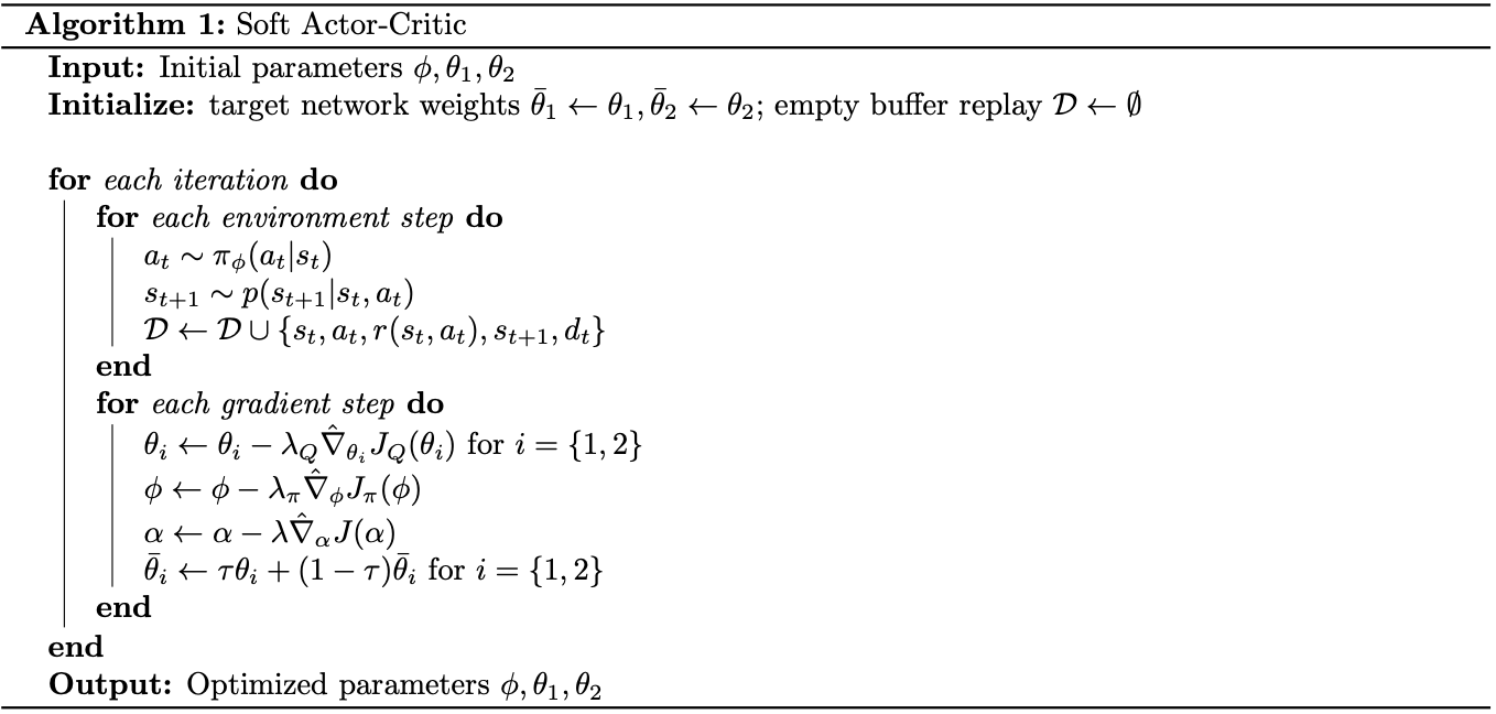
Soft Actor-Critic

In large scale problems, it is impractical to run either policy evaluation or policy improvement until convergence. It is then necessary to use an approximation version of soft policy iteration, which we call Soft Actor-Critic, or SAC. SAC instead uses function approximators (neural network function approximation is our choice) for both the policy and the soft Q-function, and rather than alternating between evaluation and improvement to convergence, using SGD to optimize both networks.

These following are key components of SAC method:

• One policy $\pi_\phi$ and two soft Q-functions $Q_{\theta_1},Q_{\theta_2}$.
• Utilizing shared target Q-networks, $Q_{\overline{\theta}_1},Q_{\overline{\theta}_2}$, whose parameters are soft updated due to \begin{equation} \bar{\theta}_i\leftarrow\tau\theta_i+(1-\tau)\bar{\theta}_i,\hspace{2cm}i=\{1,2\} \end{equation} where $\tau\in(0,1]$ and close to $0$.
• Off-policy training with samples from a replay buffer $\mathcal{D}$ to minimize correlations between samples. The rollout phase is given as for each step $t$ \begin{align*} &a_t\sim\pi_\phi(a_t\vert s_t) \\ &s_{t+1}\sim p(s_{t+1}\vert s_t,a_t) \\ &\mathcal{D}\leftarrow\mathcal{D}\cup\{s_t,a_t,r(s_t,a_t),s_{t+1},d_t\}, \end{align*} where $d_t$ informs whether $s_{t+1}$ is the terminal state.
• The Q-function parameters are trained to minimize the Mean Square Bellman Error (MSBE) \begin{equation} J_Q(\theta)=\mathbb{E}_{(s_t,a_t)\sim\mathcal{D}}\left[\frac{1}{2}\Big(y_t-Q_\theta(s_t,a_t)\Big)^2\right], \end{equation} where $y_t$ is the TD target at step $t$, which is given by \begin{align} y_t&=r(s_t,a_t)+\gamma\mathbb{E}_{s_{t+1}\sim p}\big[V_\overline{\theta}(s_{t+1})\big]\label{eq:sac.6} \\ &=r(s_t,a_t)+\gamma\mathbb{E}_{s_{t+1}\sim p,a_{t+1}\sim\pi_\phi}\Big[Q_\overline{\theta}(s_{t+1},a_{t+1})+\alpha H\big(\pi_\phi(\cdot\vert s_{t+1})\big)\Big] \\ &=r(s_t,a_t)+\gamma\mathbb{E}_{s_{t+1}\sim p,a_{t+1}\sim\pi_\phi}\Big[Q_\overline{\theta}(s_{t+1},a_{t+1})-\alpha\log\pi_\phi(a_{t+1}\vert s_{t+1})\Big], \end{align} which, as an expectation, can be approximated with samples from replay buffer $\mathcal{D}$ (i.e. $s_{t+1}\sim\mathcal{D}$ since $s_{t+1}\sim p(s_{t+1}\vert s_t,a_t)$ while $(s_t,a_t)\sim\mathcal{D}$, which is the reason why we attached $s_{t+1}$ in the replay buffer $\mathcal{D}$ as in the key point (3)) with current policy $\pi_\phi$ (i.e. $a_{t+1}\sim\pi_\phi$): \begin{equation} y_t\approx r(s_t,a_t)+\gamma\big(Q_\overline{\theta}(s_{t+1},a_{t+1})-\alpha\log\pi_\phi(a_{t+1}\vert s_{t+1})\big) \end{equation} Therefore, the loss function for Q-networks at step $t$ is given by \begin{equation} J_Q(\theta)=\mathbb{E}_{(s_t,a_t,r,s_{t+1},d_t)\sim\mathcal{D},a_{t+1}\sim\pi_\phi}\left[\frac{1}{2}\big(y(r,s_{t+1},a_{t+1},d_t)-Q_\theta(s_t,a_t)\big)^2\right],\label{eq:sac.1} \end{equation} where \begin{equation} y(r,s_{t+1},a_{t+1},d_t)=r+\gamma(1-d_t)\big(Q_\overline{\theta}(s_{t+1},a_{t+1})-\alpha\log\pi_\phi(a_{t+1}\vert s_{t+1})\big)\label{eq:sac.2} \end{equation} The loss function $J_Q(\theta)$ in \eqref{eq:sac.1} then can be optimized according to SGD using \begin{equation} \hat{\nabla}_\theta J_Q(\theta)=\nabla_\theta Q_\theta(s_t,a_t)\big(y_t-Q_\theta(s_t,a_t)\big),\label{eq:sac.3} \end{equation} where $y_t$ is the TD target at time-step $t$, which can be computed according \eqref{eq:sac.2}.
• The policy, in each state, acts greedily as \eqref{eq:gp.1}, which maximizes the expected entropy-augmented return, which is $V_\pi(s)$ \begin{align} V_\pi(s)&=\mathbb{E}_{a\sim\pi}\Big[Q_\pi(s,a)+\alpha H\big(\pi(\cdot\vert s)\big)\Big] \\ &=\mathbb{E}_{a\sim\pi}\Big[Q_\pi(s,a)-\alpha\log\pi(a\vert s)\Big] \end{align} Hence, the policy parameters $\phi$ can be learned by directly maximizing \begin{align} J_\pi(\phi)&=\mathbb{E}_{s_t\sim\mathcal{D}}\Big[\mathbb{E}_{a_t\sim\pi_\phi}\big[Q_\theta(s_t,a_t)-\alpha\log\pi_\phi(a_t\vert s_t)\big]\Big] \\ &=\mathbb{E}_{s_t\sim\mathcal{D},a_t\sim\pi_\phi}\Big[Q_\theta(s_t,a_t)-\alpha\log\pi_\phi(a_t\vert s_t)\Big]\label{eq:sac.4} \end{align} Since Q-function is represented by a neural network and can be differentiated, in SAC paper, the authors make use of the reparameterization trick to reduce variance. In particular, samples are obtained according to \begin{equation} a_\phi(s_t,\epsilon_t)=\text{tanh}(\mu_\phi(s_t)+\sigma_\phi(s_t)\odot\epsilon_t) \end{equation} where $\epsilon_t\sim\mathcal{N}(0,I)$ is a spherical Gaussian noise, $\mu_\phi$ and $\sigma_\phi$ are defined as given in the next key point. The loss function in \eqref{eq:sac.4} then can be rewritten as \begin{equation} J_\pi(\phi)=\mathbb{E}_{s_t\sim\mathcal{D},\epsilon_t\sim\mathcal{N}(0,I)}\Big[Q_\theta\big(s_t,a_\phi(s_t,\epsilon_t)\big)-\alpha\log\pi_\phi\big(a_\phi(s_t,\epsilon_t)\vert s_t\big)\Big], \end{equation} which rather than taking the expectation over actions ($a_t\sim\pi_\phi$, depends on $\phi$), computing over noise ($\epsilon_t\sim\mathcal{N}(0,I)$, depends on nothing). This function can be optimized with SGD with \begin{equation} \hspace{-0.9cm}\hat{\nabla}_\phi J_\pi(\phi)=\big(\nabla_{a_t}Q_\theta(s_t,a_t)-\alpha\nabla_{a_t}\log\pi_\phi(a_t\vert s_t)\big)\nabla_\phi a_\phi(s_t,\epsilon_t)-\alpha\nabla_\phi\log\pi_\phi(a_t\vert s_t),\label{eq:sac.5} \end{equation} where $a_t$ is evaluated at $a_\phi(s_t,\epsilon_t)$.
• For continuous action space tasks, a stochastic policy is usually given in form of a diagonal Gaussian, i.e. \begin{equation} \pi_\phi(\cdot\vert s)=\mathcal{N}(\mu_\phi(s),\Sigma_\phi(s))=\mathcal{N}(\mu_\phi(s),\sigma_\theta(s)^2 I)=\mu_\phi(s)+\sigma_\phi(s)\mathcal{N}(0,I) \end{equation} hence, when sampling from $\pi_\phi$, let $\epsilon_t\sim\mathcal{N}(0,I)$ be a vector of spherical Gaussian noise, an action $a_t\sim\mathcal{N}(\mu_\theta(s),\sigma_\phi(s)^2 I)$ can be computed as \begin{equation} a_t=\mu_\phi(s_t)+\sigma_\phi(s_t)\odot\epsilon_t, \end{equation} where $\odot$ denotes the elementwise product of two vectors.
  Since the normal distribution taking range of $(-\infty,\infty)$, it is necessary to bound the policy to a finite interval, which can be performed by applying a squashing function (e.g. $\text{tanh}$, sigmoid, etc) to the Gaussian samples. For instance, the $\text{tanh}$ function converts support of $(-\infty,\infty)$ into $(-1,1)$.
• Two soft Q-functions $Q_{\theta_1},Q_{\theta_2}$ are trained independently to optimize $J_Q(\theta_1),J_Q(\theta_2)$ respectively. Also, the minimum of the soft Q-functions is used in \eqref{eq:sac.3} and \eqref{eq:sac.5} instead, i.e. \begin{align} \hat{\nabla}_\theta J_Q(\theta)&=\nabla_\theta Q_\theta(s_t,a_t)\big(y_t-Q_\theta(s_t,a_t)\big), \\ \hat{\nabla}_\phi J_\pi(\phi)&=\big(\nabla_{a_t}\min_{i=1,2}Q_{\theta_i}(s_t,a_t)-\alpha\nabla_{a_t}\log\pi_\phi(a_t\vert s_t)\big)\nabla_\phi a_\phi(s_t,\epsilon_t)\nonumber \\ &\hspace{2cm}-\alpha\nabla_\phi\log\pi_\phi(a_t\vert s_t) \end{align} where \begin{equation} y_t=r+\gamma(1-d_t)\left(\min_{i=1,2}Q_{\overline{\theta}_i}(s_{t+1},a_{t+1})-\alpha\log\pi_\phi(a_{t+1}\vert s_{t+1})\right) \end{equation}
• Instead of considering entropy coefficient $\alpha$ as a constant, in the latter version of SAC, authors treated it as a parameter and can be optimized due to the loss function \begin{equation} J(\alpha)=\mathbb{E}_{a_t\sim\pi_t}\big[-\alpha\log\pi_t(a_t\vert s_t)-\alpha\bar{H}\big]\label{eq:sac.7} \end{equation} where $\pi_t$ denotes the current policy at time-step $t$ and $\bar{H}$ is target entropy value, usually is set as $-\text{dim}(\mathcal{A})$.

Pseudocode for our final algorithm is given below.

Discrete SAC

In discrete-action setting, the policy $\pi_\phi(a\vert s)$ can be consider as a PFM (probability mass function), instead of a density function in the continuous case. This gives rise to some necessary changes:

• We use a Categorical policy instead of a diagonal Gaussian, i.e. $\pi:\mathcal{S}\to[0,1]^{\vert\mathcal{A}\vert}$.
• The PMF-form policy allows us to compute the soft value function directly instead of using Monte Carlo sampling, i.e. \begin{equation} V_\pi(s)=\sum_{a\in\mathcal{A}}\pi(a\vert s)\big[Q_\pi(s,a)-\alpha\log\pi(a\vert s)\big],\label{eq:dsac.1} \end{equation} which reduces the variance in Monte Carlo estimate of the $V_\overline{\theta}(s_{t+1})$ given in \eqref{eq:sac.6} that is used to compute the loss function of Q-networks $J_Q(\theta)$.
  It is then more efficient to make a modification to the soft Q-function: The soft Q-function returns a value for each possible action rather than simply the action provided as an input, i.e. $Q:\mathcal{S}\to\mathbb{R}^{\vert\mathcal{A}\vert}$.
  This change, along with the previous one, lets us rewrite the calculation for soft state-value given in \eqref{eq:dsac.1} as \begin{equation} V_\pi(s)=\pi(s)^\text{T}\big[Q_\pi(s)-\alpha\log\pi(s)\big] \end{equation}
• Analogously, the entropy coefficient loss changes from \eqref{eq:sac.7} to \begin{equation} J(\alpha)=\pi_t(s_t)^\text{T}\big[-\alpha\log\pi_t(s_t)-\alpha\bar{H}\big] \end{equation}
• Since the policy $\pi$ now returns the exact action, we are able to compute the expectation directly. Thus, it is unnecessary to use the reparameterization trick in the calculation for the loss function $J_\pi(\phi)$. It is then given by \begin{equation} J_\pi(\phi)=\mathbb{E}_{s_t\sim\mathcal{D}}\Big[\pi_\phi(s_t)^\text{T}\big[Q_\theta(s_t)-\alpha\log\pi_\phi(s_t)\big]\Big] \end{equation}

Soft Q-learning

References

[1] Tuomas Haarnoja, Haoran Tang, Pieter Abbeel, Sergey Levine. Reinforcement Learning with Deep Energy-Based Policies. ICML, 2017.

[2] Tuomas Haarnoja, Aurick Zhou, Pieter Abbeel, Sergey Levine. Soft Actor-Critic: Off-Policy Maximum Entropy Deep Reinforcement Learning with a Stochastic Actor. arXiv preprint, arXiv:1812.05905, 2018.

[3] Tuomas Haarnoja, Aurick Zhou, Kristian Hartikainen, George Tucker, Sehoon Ha, Jie Tan, Vikash Kumar, Henry Zhu, Abhishek Gupta, Pieter Abbeel, Sergey Levine. Soft Actor-Critic Algorithms and Applications. arXiv preprint, arXiv:1812.05905, 2019.

[4] Brian D. Ziebart. Modeling purposeful adaptive behavior with the principle of maximum causal entropy. PhD Thesis, Carnegie Mellon University, 2010.

[5] John Schulman, Xi Chen, Pieter Abbeel. Equivalence Between Policy Gradients and Soft Q-Learning. arXiv preprint arXiv:1704.06440, 2018.

[6] Csaba Szepesvári. Algorithms for Reinforcement Learning. Synthesis Lectures on Artificial Intelligence and Machine Learning, 2010.

[7] Richard S. Sutton, Andrew G. Barto. Reinforcement Learning: An Introduction. MIT press, 2018.

[8] Josh Achiam. Spinning Up in Deep Reinforcement Learning. SpinningUp2018, 2018.

[9] Petros Christodoulou. Soft Actor-Critic for Discrete Action Settings. arXiv preprint, arXiv:1910.07207.

Footnotes