Multi-agent Deep Deterministic Policy Gradient

Notes on MADDPG.

Preliminaries

Markov Games

A partially observable Markov game for $N$ agents is defined by a set of states $\mathcal{S}$, an action set $\mathcal{A}_1,\ldots,\mathcal{A}_N$ and an observation set $\mathcal{O}_1,\ldots,\mathcal{O}_N$ for each agent. Also, let $\rho:\mathcal{S}\mapsto[0,1]$ denote the initial state distribution.

To choose actions, each agent $i$ uses a stochastic policy $\pi_{\theta_i}:\mathcal{O}_i\times\mathcal{A}_i\mapsto[0,1]$, which produces the next state according to the state transition function $\mathcal{T}:\mathcal{S}\times\mathcal{A}_1\times\ldots\times\mathcal{A}_N\mapsto\mathcal{S}$.

For each action taken, each agent $i$ obtains rewards $r_i:\mathcal{S}\times\mathcal{A}_i\mapsto\mathbb{R}$ and a private observation correlated with the state $o_i:\mathcal{S}\mapsto\mathcal{O}_i$.

The goal of each agent $i$ to maximize its own total expected return \begin{equation} J(\theta_i)=\mathbb{E}_{\pi_{\theta_i}}[R_i]=\mathbb{E}_{\pi_{\theta_i}}\left[\sum_{t=0}^{T}\gamma^t r_i^t\right], \end{equation} where $\gamma$ is a discount factor and $T$ is the time horizon.

Q-Learning and DQN

Q-Learning iteratively updates the state-action value function $Q^\pi(s,a)=\mathbb{E}\big[R\vert s_t=s,a_t=a\big]$ of policy $\pi$ as \begin{equation} Q^\pi(s,a)=\mathbb{E}_{s’}\Big[r(s,a)+\gamma\mathbb{E}_{a’\sim\pi}\big[Q^\pi(s’,a’)\big]\Big] \end{equation} DQN utilizes a target network and an experience replay buffer to extend the idea of Q-Learning update with neural networks. In particular, it learns a Q-network parameterized by $\theta$, $Q_\theta$ by minimizing the loss \begin{equation} \mathcal{L}(\theta_t)=\mathbb{E}_{s,a,r,s’}\Big[\big(Q_{\theta_t}^*(s,a)-y_t\big)^2\Big], \end{equation} where $y$ is referred as the TD target, defined as \begin{equation} y=r+\gamma\max_{a’}\hat{Q}_{\theta_{t-1}}(s’,a’) \end{equation}

Policy Gradients

Policy gradient methods are policy optimization algorithms with the key idea is to adjust the parameters $\theta$ of the policy $\pi$ in order to maximize $J(\theta)=\mathbb{E}_{s\sim\rho^\pi,a\sim\pi_\theta}[R]$ by taking step in the direction of its gradient, called the policy gradient. Specifically, recall that in the case of stochastic policy, the Policy Gradient Theorem states that¹ \begin{align} \nabla_\theta J(\theta)&=\int_\mathcal{S}\rho^\pi(s)\int_\mathcal{A}\nabla_\theta\pi_\theta(a\vert s)Q^\pi(s,a)\hspace{0.1cm}da\hspace{0.1cm}ds \\ &=\mathbb{E}_{s\sim\rho^\pi,a\sim\pi_\theta}\Big[\nabla_\theta\log\pi_\theta(a\vert s)Q^\pi(s,a)\Big], \end{align} where $\rho^\pi$ is the state distribution, indicate how often the state occurs under the policy $\pi$.

Deterministic Policy Gradient

The Policy Gradient Theorem can also extend to deterministic policies, which results the Deterministic Policy Gradient Theorem. Specifically, consider a deterministic policy $\mu_\theta:\mathcal{S}\mapsto\mathcal{A}$, the policy gradient, or the gradient of the objective function $J(\theta)=\mathbb{E}_{s\sim\rho^\mu}[R(s,a)]$ has the form of \begin{align} \nabla_\theta J(\theta)&=\int_\mathcal{S}\rho^\mu(s)\nabla_\theta\mu_\theta(s)\nabla_a Q^\mu(s,a)\big\vert_{a=\mu_\theta(s)}\hspace{0.1cm}ds \\ &=\mathbb{E}_{s\sim\mathcal{D}}\Big[\nabla_\theta\mu_\theta(a\vert s)\nabla_a Q^\mu(s,a)\big\vert_{a=\mu_\theta(s)}\Big], \end{align} where the action space $\mathcal{A}$ must be continuous (and thus the policy $\mu$) for $\nabla_a Q^\mu(s,a)$ to exist.

Multi-agent DDPG

Multi-agent Actor-Critic

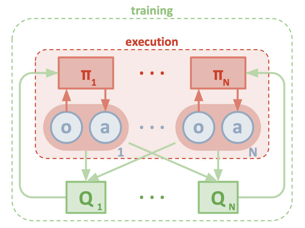
Consider a game of $N$ agents, each corresponds to a policy of $\boldsymbol{\pi}=\{\pi_1,\ldots,\pi_N\}$, where the policies are parameterized by $\boldsymbol{\theta}=\{\theta_1,\ldots,\theta_N\}$. The gradient of the expected return for agent $i$, $J(\theta_i)$, can be written as \begin{equation} \nabla_{\theta_i}J(\theta_i)=\mathbb{E}_{s\sim\rho^\boldsymbol{\pi},a_i\sim\pi_i}\Big[\nabla_{\theta_i}\log\pi_i(a_i\vert o_i)Q_i^\boldsymbol{\pi}(\mathbf{x},a_1,\ldots,a_N)\Big]\label{eq:maddpg.1} \end{equation} The Q-function, $Q_i^\boldsymbol{\pi}(\mathbf{x},a_1,\ldots,a_N)$, is a centralized action-value function since it takes as input the actions of all agents, $a_1,\ldots,a_N$, and some state information $\mathbf{x}$, and outputs the action-value function for agent $i$.

We can apply this idea for the case of deterministic policies. In particular, let us consider $N$ continuous deterministic policies $\mu_{\theta_i}:\mathcal{S}\mapsto\mathcal{A}_i$ with $i=1,\ldots,N$ (or $\mu_i$ for short). The gradient in \eqref{eq:maddpg.1} then can be rewritten as \begin{equation} \nabla_{\theta_i}J(\theta_i)=\mathbb{E}_{\mathbf{x},a\sim\mathcal{D}}\Big[\nabla_{\theta_i}\boldsymbol{\mu}_i(a_i\vert o_i)\nabla_{a_i}Q_i^\boldsymbol{\mu}(\mathbf{x},a_1,\ldots,a_N)\big\vert_{a_i=\mu_i(o_i)}\Big], \end{equation} where the experience replay buffer $\mathcal{D}$ contains the tuples $(\mathbf{x},\mathbf{x}’,a_1,\ldots,a_N,r_1,r_N)$, recording experiences of all agents. The centralized action-value function $Q_i^\boldsymbol{\mu}$ is updated as \begin{equation} \mathcal{L}(\theta_i)=\mathbb{E}_{\mathbf{x},a,r,\mathbf{x}’}\Big[\big(Q_i^\boldsymbol{\mu}(\mathbf{x},a_1,\ldots,a_N)-y\big)^2\Big],\label{eq:maddpg.2} \end{equation} where \begin{equation} y=r_i+\gamma Q_i^{\boldsymbol{\mu}’}(\mathbf{x}’,a_1’,\ldots,a_N’)\big\vert_{a_j’=\mu_j’(o_j)}, \end{equation} where $\boldsymbol{\mu}’\doteq\{\mu_1’,\ldots,\mu_N’\}=\{\mu_{\theta_1}’,\ldots,\mu_{\theta_N}’\}$ is the set of all target policies with delayed parameters $\theta_i’$.

Note that to perform the update in \eqref{eq:maddpg.2}, we require the policies of other agents. We can relax this assumption by learning the policies of other agents from observations.

Inferring policies of other agents

To remove the assumption of acknowledge about other agents’ policies, each agent $i$ can additionally maintain an approximation $\hat{\mu}_{\phi_i^j}$ (or $\hat{\mu}_i^j$ for short, where $\phi$ are the parameters of the approximation) to the true policy of agent $j$, $\mu_j$. This approximate policy is learned through maximizing the log probability of agent $j$’s actions, with an entropy regularizer \begin{equation} \mathcal{L}(\phi_i^j)=-\mathbb{E}_{o_j,a_j}\Big[\log\hat{\mu}_i^j(a_j\vert o_j)+\lambda H(\hat{\mu}_i^j)\Big],\label{eq:maddpg.3} \end{equation} where $H$ is the entropy of the policy distribution. Given the approximate policies, we can rewrite the update in \eqref{eq:maddpg.2} as \begin{equation} \mathcal{L}(\theta_i)=\mathbb{E}_{\mathbf{x},a,r,\mathbf{x}’}\Big[\big(Q_i^\boldsymbol{\mu}(\mathbf{x},a_1,\ldots,a_N)-\hat{y}\big)^2\Big], \end{equation} where \begin{equation} \hat{y}=r_i+\gamma Q_i^{\boldsymbol{\mu}’}\big(\mathbf{x}’,{\hat{\mu}’}_i^1(o_1),\ldots,\mu_i’(o_i),\ldots,{\hat{\mu}’}_N^1(o_N)\big), \end{equation} where ${\hat{\mu}’}_i^j$ denotes the target network for the approximate policy $\hat{\mu}_i^j$.

Note that each loss function, $\mathcal{L}(\phi_i^j)$, given in \eqref{eq:maddpg.3} can be optimized in online fashion, in the sense that before updating $Q_i^\boldsymbol{\mu}$, we take the latest samples of each agent $j$ from the replay buffer $\mathcal{D}$ to perform a single gradient step to update $\phi_i^j$.

Agents with policy ensembles

At each step, we randomly select one particular sub-policy for each agent to execute. Suppose that policy $\mu_i$ is an ensemble of $K$ different sub-policies $\mu_{\theta_i^{(k)}}$ (or $\mu_i^{(k)}$ in short). For agent $i$, we are then maximizing the ensemble objective \begin{equation} J_e(\mu_i)=\mathbb{E}_{k\sim\text{Unif}(1,K),s\sim\rho^\boldsymbol{\mu},a\sim\mu_i^{(k)}}\big[R_i(s,a)\big] \end{equation} Since different sub-policies will be executed in different episodes, we maintain a replay buffer $\mathcal{D}_i^{(k)}$ for each sub-policy $\mu_i^{(k)}$ of agent $i$. The gradient of the ensemble objective $J_e(\mu_i)$ w.r.t $\theta_i^{(k)}$ can be derive as \begin{equation} \nabla_{\theta_i^{(k)}}J_e(\mu_i)=\frac{1}{K}\mathbb{E}_{\mathbf{x},a\sim\mathcal{D}_i^{(k)}}\Big[\nabla_{\theta_i^{(k)}}\mu_i^{(k)}(a_i\vert o_i)\nabla_{a_i}Q^{\mu_i}(\mathbf{x},a_1,\ldots,a_N)\big\vert_{a_i=\mu_i^{(k)}(o_i)}\Big] \end{equation}

References

[1] Ryan Lowe, Yi Wu, Aviv Tamar, Jean Harb, Pieter Abbeel, Igor Mordatch. Multi-Agent Actor-Critic for Mixed Cooperative-Competitive Environments. NIPS 2017.

[2] David Silver, Guy Lever, Nicolas Heess, Thomas Degris, Daan Wierstra, Martin Riedmiller. Deterministic Policy Gradient Algorithms. JMLR 2014.

[3] Richard S. Sutton, Andrew G. Barto. Reinforcement Learning: An Introduction. MIT press, 2018.

[4] Richard S. Sutton, David McAllester, Satinder Singh, Yishay Mansour. Policy Gradient Methods for Reinforcement Learning with Function Approximation. NIPS 1999.

Footnotes