Function Approximation

All of the tabular methods we have been considering so far might scale well within a small state space. However, when dealing with Reinforcement Learning problems in continuous state space, an exact solution is nearly impossible to find. But instead, an approximated answer could be found.

On-policy Methods

So far in the series, we have gone through tabular methods, which are used to solve problems with small state and action spaces. For larger spaces, rather than getting the exact solutions, we now have to approximate the value of them. To start, we begin with on-policy approximation methods.

Value-function Approximation

All of the prediction methods so far have been described as updates to an estimated value function that shift its value at particular states toward a “backed-up value” (or update target) for that state \begin{equation} s\mapsto u, \end{equation} where $s$ is the state updated and $u$ is the update target that $s$’s estimated value is shifted toward.

For example,

• the MC update for value prediction is: $S_t\mapsto G_t$.
• the TD(0) update for value prediction is: $S_t\mapsto R_{t+1}+\gamma\hat{v}(S_{t+1},\mathbf{w}_t)$.
• the $n$-step TD update is: $S_t\mapsto G_{t:t+n}$.
• and in the DP, policy-evaluation update, $s\mapsto\mathbb{E}\big[R_{t+1}+\gamma\hat{v}(S_{t+1},\mathbf{w}_t)\vert S_t=s\big]$, an arbitrary $s$ is updated.

Each update $s\mapsto u$ can be viewed as example of the desired input-output behavior of the value function. And when the outputs are numbers, like $u$, we call the process function approximation.

The Prediction Objective

In contrast to tabular case, where the solution of value function could be found equal to the true value function exactly, and an update at one state did not affect the others, with function approximation, it is impossible to find the exact value function of all states. And moreover, an update at one state also affects many others.

Hence, it is necessary to specify a state distribution $\mu(s)\geq0,\sum_s\mu(s)=1$, representing how much we care about the error (the difference between the approximate value $\hat{v}(s,\mathbf{w})$ and the true value $v_\pi(s)$) in each state $s$. Weighting this over the state space $\mathcal{S}$ by $\mu$, we obtain a natural objective function, called the Mean Squared Value Error, denoted as $\overline{\text{VE}}$: \begin{equation} \overline{\text{VE}}(\mathbf{w})\doteq\sum_{s\in\mathcal{S}}\mu(s)\Big[v_\pi(s)-\hat{v}(s,\mathbf{w})\Big]^2 \end{equation} The distribution $\mu(s)$ is usually chosen as the fraction of time spent in $s$ (number of time $s$ visited divided by total amount of visits). Under on-policy training this is called the on-policy distribution.

• In continuing tasks, the on-policy distribution is the stationary distribution under $\pi$.
• In episodic tasks, the on-policy distribution depends on how the initial states are chosen.
  • Let $h(s)$ denote the probability that an episode begins in each state $s$, and let $\eta(s)$ denote the number of time steps spent, on average, in state $s$ in a single episode \begin{equation} \eta(s)=h(s)+\sum_\bar{s}\eta(\bar{s})\sum_a\pi(a\vert\bar{s})p(s\vert\bar{s},a),\hspace{1cm}\forall s\in\mathcal{S} \end{equation} This system of equation can be solved for the expected number of visits $\eta(s)$. The on-policy distribution is then \begin{equation} \mu(s)=\frac{\eta(s)}{\sum_{s’}\eta(s’)},\hspace{1cm}\forall s\in\mathcal{S} \end{equation}

Gradient-based algorithms

To solve the least squares problem, we are going to use a popular method, named Gradient descent.

Say, consider a differentiable function $J(\mathbf{w})$ of parameter vector $\mathbf{w}$.

The gradient of $J(\mathbf{w})$ w.r.t $\mathbf{w}$ is defined to be \begin{equation} \nabla_{\mathbf{w}}J(\mathbf{w})=\left(\begin{smallmatrix}\dfrac{\partial J(\mathbf{w})}{\partial\mathbf{w}_1} \\ \vdots \\ \dfrac{\partial J(\mathbf{w})}{\partial\mathbf{w}_d}\end{smallmatrix}\right) \end{equation} The idea of Gradient descent is to minimize the objective function $J(\mathbf{w})$, we repeatedly move $\mathbf{w}$ in the direction of steepest decrease of $J$, which is the direction of negative gradient $-\nabla_\mathbf{w}J(\mathbf{w})$.

Thus, we have the update rule of Gradient descent: \begin{equation} \mathbf{w}:=\mathbf{w}-\dfrac{1}{2}\alpha\nabla_\mathbf{w}J(\mathbf{w}), \end{equation} where $\alpha$ is a positive step-size parameter.

Stochastic-gradient

Apply gradient descent to our problem, which is we have to find the minimization of \begin{equation} \overline{\text{VE}}(\mathbf{w})=\sum_{s\in\mathcal{S}}\mu(s)\Big[v_\pi(s)-\hat{v}(s,\mathbf{w})\Big]^2 \end{equation} Since $\mu(s)$ is the state distribution over state space $\mathcal{S}$, we can rewrite $\overline{\text{VE}}$ as \begin{equation} \overline{\text{VE}}(\mathbf{w})=\mathbb{E}_{s\sim\mu}\Big[v_\pi(s)-\hat{v}(s,\mathbf{w})\Big]^2 \end{equation} By the update we have defined earlier, in each step, we need to decrease $\mathbf{w}$ by an amount of \begin{equation} \Delta\mathbf{w}=-\dfrac{1}{2}\alpha\nabla_\mathbf{w}\overline{\text{VE}}(\mathbf{w})=\alpha\mathbb{E}\Big[v_\pi(s)-\hat{v}(s,\mathbf{w})\Big]\nabla_\mathbf{w}\hat{v}(s,\mathbf{w}) \end{equation} Assume that, on each step, we observe a new example $S_t\mapsto v_\pi(S_t)$ consisting of a state $S_t$ and its true value under the policy $\pi$.

Using Stochastic Gradient descent (SGD), we adjust the weight vector after each example by a small amount in the direction that would most reduce the error on that example: \begin{align} \mathbf{w}_{t+1}&\doteq\mathbf{w}_t-\frac{1}{2}\alpha\nabla_\mathbf{w}\big[v_\pi(S_t)-\hat{v}(S_t,\mathbf{w}_t)\big]^2 \\ &=\mathbf{w}_t+\alpha\big[v_\pi(S_t)-\hat{v}(S_t,\mathbf{w}_t)\big]\nabla_\mathbf{w}\hat{v}(S_t,\mathbf{w}_t)\label{eq:sg.1} \end{align} When the target output, here denoted as $U_t\in\mathbb{R}$, of the $t$-th training example, $S_t\mapsto U_t$, is not the true value, $v_\pi(S_t)$, but some approximation to it, we cannot perform the exact update \eqref{eq:sg.1} since $v_\pi(S_t)$ is unknown, but we can approximate it by substituting $U_t$ in place of $v_\pi(S_t)$. This yield the following general SGD method for state-value prediction: \begin{equation} \mathbf{w}_{t+1}\doteq\mathbf{w}_t+\alpha\big[U_t-\hat{v}(S_t,\mathbf{w}_t)\big]\nabla_\mathbf{w}\hat{v}(S_t,\mathbf{w}_t)\label{eq:sg.2} \end{equation} If $U_t$ is an unbiased estimate of $v_\pi(S_t)$, i.e., $\mathbb{E}\left[U_t\vert S_t=s\right]=v_\pi(S_t)$, for each $t$, then $\mathbf{w}_t$ is guaranteed to converge to a local optimum under the usual stochastic conditions for decreasing $\alpha$.

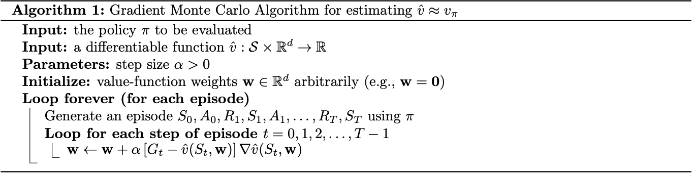
In particular, since the true value of a state is the expected value of the return following it, the Monte Carlo target $U_t\doteq G_t$, we have that the SGD version of Monte Carlo state-value prediction, \begin{equation} \mathbf{w}_{t+1}\doteq\mathbf{w}_t+\alpha\big[G_t-\hat{v}(S_t,\mathbf{w}_t)\big]\nabla_\mathbf{w}\hat{v}(S_t,\mathbf{w}_t), \end{equation} is guaranteed to converge to a local optimal point.

We have the pseudocode of the algorithm

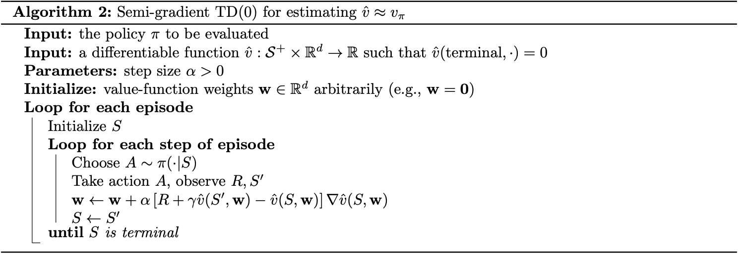
Semi-gradient

If instead of using MC target $G_t$, we use the bootstrapping targets such as $n$-step return $G_{t:t+n}$ or the DP target $\sum_{a,s’,r}\pi(a\vert S_t)p(s’,r\vert S_t,a)\left[r+\gamma\hat{v}(s’,\mathbf{w}_t)\right]$, which all depend on the current value of the weight vector $\mathbf{w}_t$, and then implies that they will be biased, and will not produce a true gradient-descent method.

Such methods are called semi-gradient since they include only a part of the gradient.

Linear Function Approximation

One of the most crucial special cases of function approximation is that in which the approximate function, $\hat{v}(\cdot,\mathbf{w})$, is a linear function of the weight vector, $\mathbf{w}$.

Corresponding to every state $s$, there is a real-valued vector $\mathbf{x}(s)\doteq\left(x_1(s),x_2(s),\dots,x_d(s)\right)$, with the same number of components with $\mathbf{w}$.

Linear Methods

Linear methods approximate value function by the inner product between $\mathbf{w}$ and $\mathbf{x}(s)$: \begin{equation} \hat{v}(s,\mathbf{w})\doteq\mathbf{w}^\text{T}\mathbf{x}(s)=\sum_{i=1}^{d}w_ix_i(s)\label{eq:lm.1} \end{equation} The vector $\mathbf{x}(s)$ is called a feature vector representing state $s$, i.e., $x_i:\mathcal{S}\to\mathbb{R}$.

For linear methods, features are basis functions because they form a linear basis for the set of approximate functions. Constructing $d$-dimensional feature vectors to represent states is the same as selecting a set of $d$ basis functions.

From \eqref{eq:lm.1}, when using SGD updates with linear approximation, we have the gradient of the approximate value function w.r.t $\mathbf{w}$ is \begin{equation} \nabla_\mathbf{w}\hat{v}(s,\mathbf{w})=\mathbf{x}(s) \end{equation} Thus, with linear approximation, the SGD update can be rewrite as \begin{equation} \mathbf{w}_{t+1}\doteq\mathbf{w}_t+\alpha\left[G_t-\hat{v}(S_t,\mathbf{w}_t)\right]\mathbf{x}(S_t) \end{equation}

In the linear case, there is only one optimum, and thus any method that is guaranteed to converge to or near a local optimum is automatically guaranteed to converge to or near the global optimum.

• The gradient MC algorithm in the previous section converges to the global optimum of the $\overline{\text{VE}}$ under linear function approximation if $\alpha$ is reduced over time according to the usual conditions. In particular, it converges to the fixed point, called $\mathbf{w}_{\text{MC}}$, with: \begin{align} \nabla_{\mathbf{w}_{\text{MC}}}\mathbb{E}\left[\big(G_t-v_{\mathbf{w}_{\text{MC}}}(S_t)\big)^2\right]&=0 \\ \mathbb{E}\Big[\big(G_t-v_{\mathbf{w}_{\text{MC}}}(S_t)\big)\mathbf{x}_t\Big]&=0 \\ \mathbb{E}\Big[(G_t-\mathbf{x}_t^\text{T}\mathbf{w}_{\text{MC}})\mathbf{x}_t\Big]&=0 \\ \mathbb{E}\left[G_t\mathbf{x}_t-\mathbf{x}_t\mathbf{x}_t^\text{T}\mathbf{w}_{\text{MC}}\right]&=0 \\ \mathbb{E}\left[\mathbf{x}_t\mathbf{x}_t^\text{T}\right]\mathbf{w}_\text{MC}&=\mathbb{E}\left[G_t\mathbf{x}_t\right] \\ \mathbf{w}_\text{MC}&=\mathbb{E}\left[\mathbf{x}_t\mathbf{x}_t^\text{T}\right]^{-1}\mathbb{E}\left[G_t\mathbf{x}_t\right] \end{align}
• The semi-gradient TD algorithm also converges under linear approximation.
  • Recall that, at each time $t$, the semi-gradient TD update is \begin{align} \mathbf{w}_{t+1}&\doteq\mathbf{w}_t+\alpha\left(R_{t+1}+\gamma\mathbf{w}_t^\text{T}\mathbf{x}_{t+1}-\mathbf{w}_t^\text{T}\mathbf{x}_t\right)\mathbf{x}_t \\ &=\mathbf{w}_t+\alpha\left(R_{t+1}\mathbf{x}_t-\mathbf{x}_t(\mathbf{x}_t-\gamma\mathbf{x}_{t+1})^\text{T}\mathbf{w}_t\right), \end{align} where $\mathbf{x}_t=\mathbf{x}(S_t)$. Once the system has reached steady state, for any given $\mathbf{w}_t$, the expected next weight vector can be written as \begin{equation} \mathbb{E}\left[\mathbf{w}_{t+1}\vert\mathbf{w}_t\right]=\mathbf{w}_t+\alpha\left(\mathbf{b}-\mathbf{A}\mathbf{w}_t\right),\label{eq:lm.2} \end{equation} where \begin{align} \mathbf{b}&\doteq\mathbb{E}\left[R_{t+1}\mathbf{x}_t\right]\in\mathbb{R}^d, \\ \mathbf{A}&\doteq\mathbb{E}\left[\mathbf{x}_t\left(\mathbf{x}_t-\gamma\mathbf{x}_{t+1}\right)^\text{T}\right]\in\mathbb{R}^d\times\mathbb{R}^d\label{eq:lm.3} \end{align} From \eqref{eq:lm.2}, it is easily seen that if the system converges, it must converges to the weight vector $\mathbf{w}_{\text{TD}}$ at which \begin{align} \mathbf{b}-\mathbf{A}\mathbf{w}_{\text{TD}}&=\mathbf{0} \\ \mathbf{w}_{\text{TD}}&=\mathbf{A}^{-1}\mathbf{b} \end{align} This quantity, $\mathbf{w}_{\text{TD}}$, is called the TD fixed point. And in fact, linear semi-gradient TD(0) converges to this point¹.
  • At the TD fixed point, it has also been proven (in the continuing case) that $\overline{\text{VE}}$ is within a bounded expansion of the lowest possible error, while the Monte Carlo solutions minimize the value error $\overline{\text{VE}}$: \begin{equation} \overline{\text{VE}}(\mathbf{w}_{\text{TD}})\leq\dfrac{1}{1-\gamma}\overline{\text{VE}}(\mathbf{w}_{\text{MC}})=\dfrac{1}{1-\gamma}\min_{\mathbf{w}}\overline{\text{VE}}(\mathbf{w}) \end{equation}

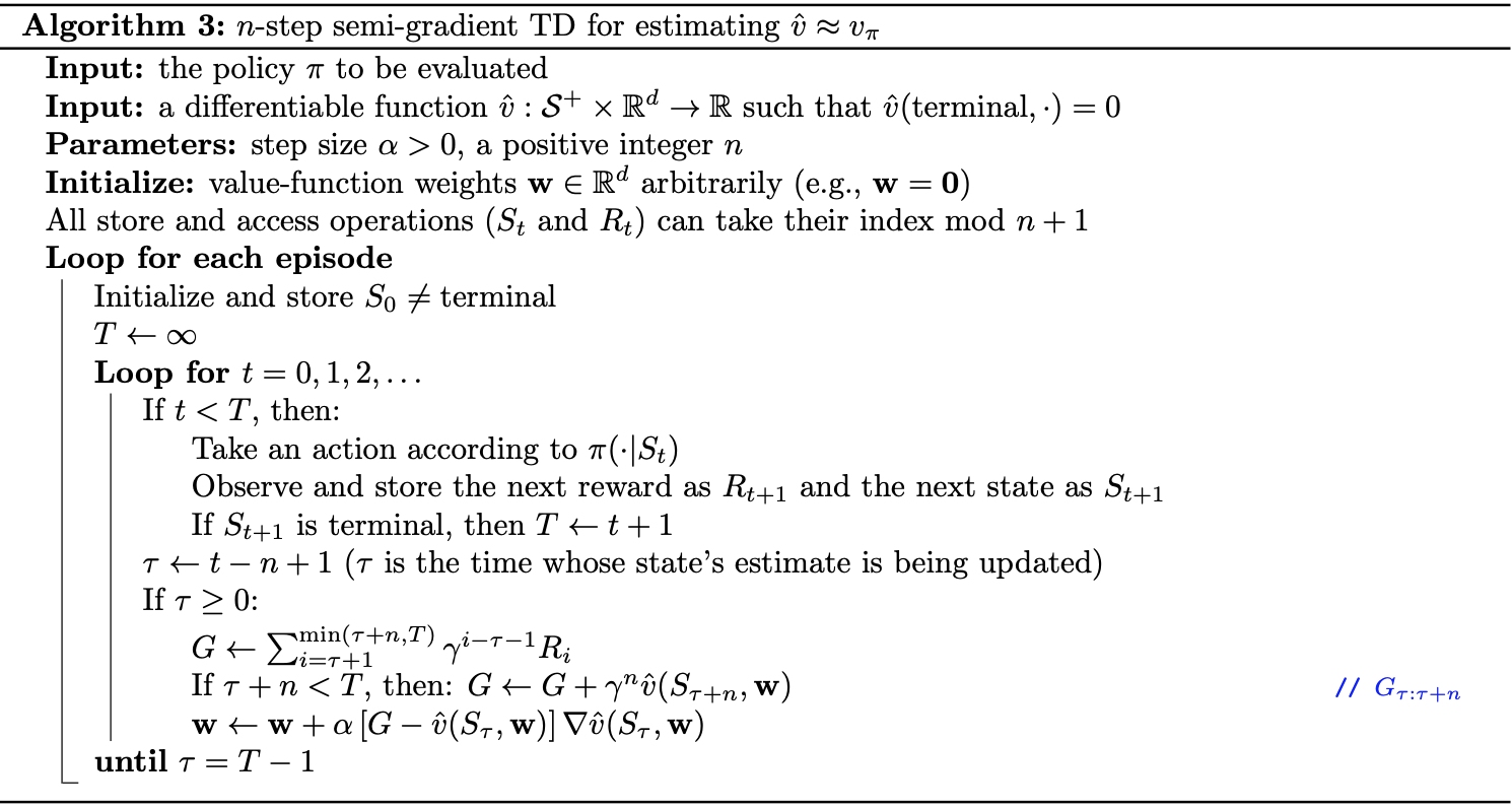
Based on the tabular $n$-step TD we have defined before, applying the semi-gradient method, we have the function approximation version of its, called semi-gradient $\boldsymbol{n}$-step TD, can be defined as: \begin{equation} \mathbf{w}_{t+n}\doteq\mathbf{w}_{t+n-1}+\alpha\left[G_{t:t+n}-\hat{v}(S_t,\mathbf{w}_{t+n-1})\right]\nabla_\mathbf{w}\hat{v}(S_t,\mathbf{w}_{t+n-1}),\hspace{1cm}0\leq t\lt T \end{equation} where the $n$-step return is generalized from the tabular version: \begin{equation} G_{t:t+n}\doteq R_{t+1}+\gamma R_{t+2}+\dots+\gamma^{n-1}R_{t+n}+\gamma^n\hat{v}(S_{t+n},\mathbf{w}_{t+n-1}),\hspace{1cm}0\geq t\geq T-n \end{equation} We therefore have the pseudocode of the semi-gradient $n$-step TD algorithm.

Feature Construction

There are various ways to define features. The simplest way is to use each variable directly as a basis function along with a constant function, i.e., setting: \begin{equation} x_0(s)=1;\hspace{1cm}x_i(s)=s_i,0\leq i\leq d \end{equation} However, most interesting value functions are too complex to be represented in this way. This scheme therefore was generalized into the polynomial basis.

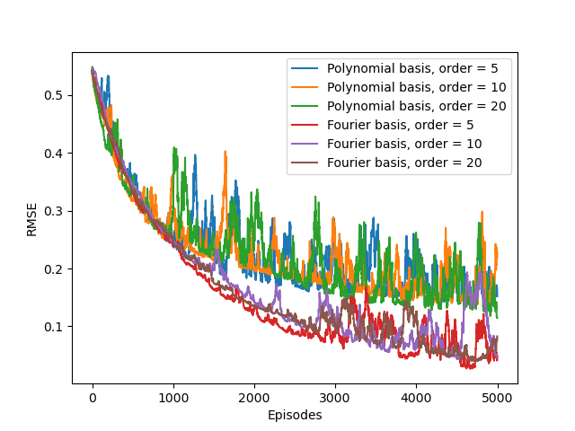
Polynomial Basis

Suppose each state $s$ corresponds to $d$ numbers, $s_1,s_2\dots,s_d$, with each $s_i\in\mathbb{R}$. For this $d$-dimensional state space, each order-$n$ polynomial basis feature $x_i$ can be written as \begin{equation} x_i(s)=\prod_{j=1}^{d}s_j^{c_{i,j}}, \end{equation} where each $c_{i,j}\in\{0,1,\dots,n\}$ for an integer $n\geq 0$. These features make up the order-$n$ polynomial basis for dimension $d$, which contains $(n+1)^d$ different features.

Fourier Basis

The Univariate Fourier Series

Fourier series is applied widely in Mathematics to approximate a periodic function². For example:

In particular, the $n$-degree Fourier expansion of $f$ with period $\tau$ is \begin{equation} \bar{f}(x)=\dfrac{a_0}{2}+\sum_{k=1}^{n}\left[a_k\cos\left(k\frac{2\pi}{\tau}x\right)+b_k\left(k\frac{2\pi}{\tau}x\right)\right], \end{equation} where \begin{align} a_k&=\frac{2}{\tau}\int_{0}^{\tau}f(x)\cos\left(\frac{2\pi kx}{\tau}\right)\hspace{0.1cm}dx, \\ b_k&=\frac{2}{\tau}\int_{0}^{\tau}f(x)\sin\left(\frac{2\pi kx}{\tau}\right)\hspace{0.1cm}dx \end{align} In the RL setting, $f$ is unknown so we cannot compute $a_0,\dots,a_n$ and $b_1,\dots,b_n$, but we can instead treat them as parameters in a linear function approximation scheme, with \begin{equation} \phi_i(x)=\begin{cases}1 &\text{if }i=0 \\ \cos\left(\frac{(i+1)\pi x}{\tau}\right) &\text{if }i>0,i\text{ odd} \\ \sin\left(\frac{i\pi x}{\tau}\right) &\text{if }i>0,i\text{ even}\end{cases} \end{equation} Thus, a full $n$-th order Fourier approximation to a one-dimensional value function results in a linear function approximation with $2n+1$ terms.

Even, Odd and Non-Periodic Functions

If $f$ is known to be even (i.e., $f(x)=f(-x)$), then $\forall i>0$, we have: \begin{align} b_i&=\frac{2}{\tau}\int_{0}^{\tau}f(x)\sin\left(\frac{2\pi ix}{\tau}\right)\hspace{0.1cm}dx \\ &=\frac{2}{\tau}\left[\int_{0}^{\tau/2}f(x)\sin\left(\frac{2\pi ix}{\tau}\right)\hspace{0.1cm}dx+\int_{\tau/2}^{\tau}f(x)\sin\left(\frac{2\pi ix}{\tau}\right)\hspace{0.1cm}dx\right] \\ &=\frac{2}{\tau}\left[\int_{0}^{\tau/2}f(x)\sin\left(\frac{2\pi ix}{\tau}\right)\hspace{0.1cm}dx+\int_{\tau/2}^{\tau}f(x-\tau)\sin\left(\frac{2\pi ix}{\tau}-2\pi i\right)\hspace{0.1cm}dx\right] \\ &=\frac{2}{\tau}\left[\int_{0}^{\tau/2}f(x)\sin\left(\frac{2\pi ix}{\tau}\right)\hspace{0.1cm}dx+\int_{\tau/2}^{\tau}f(x-\tau)\sin\left(\frac{2\pi i(x-\tau)}{\tau}\right)\hspace{0.1cm}dx\right] \\ &=\frac{2}{\tau}\left[\int_{0}^{\tau/2}f(x)\sin\left(\frac{2\pi ix}{\tau}\right)\hspace{0.1cm}dx+\int_{-\tau/2}^{0}f(x)\sin\left(\frac{2\pi ix}{\tau}\right)\hspace{0.1cm}dx\right] \\ &=0, \end{align} so the $\sin$ terms can be dropped, which reduces the terms required for an $n$-th order Fourier approximation to $n+1$.

Similarly, if $f$ is known to be odd (i.e., $f(x)=-f(-x)$), then $\forall i>0, a_i=0$, so we can omit the $\cos$ terms.

However, in general, value functions are not even, odd, or periodic (or known to be in advance). In such cases, if $f$ is defined over a bounded interval with length, let us assume, $\tau$, or without loss of generality, $\left[-\frac{\tau}{2},\frac{\tau}{2}\right]$, but only project the input variable to $\left[0,\frac{\tau}{2}\right]$. This results in a function periodic on $\left[-\frac{\tau}{2},\frac{\tau}{2}\right]$, but unconstrained on $\left(0,\frac{\tau}{2}\right]$. We are now free to choose whether or not the function is even or odd over $\left[-\frac{\tau}{2},\frac{\tau}{2}\right]$, and can drop half of the terms in the approximation.

In general, we expect it will be better to use the “half-even” approximation and drop the $\sin$ terms because this causes only a slight discontinuity at the origin. Thus, we can define the univariate $n$-th order Fourier basis as: \begin{equation} x_i(s)=\cos(i\pi s), \end{equation} for $i=0,\dots,n$.

The Multivariate Fourier Series

The $n$-order Fourier expansion of the multivariate function $F$ with period $\tau$ in $d$ dimensions is \begin{equation} \overline{F}(\mathbf{x})=\sum_\mathbf{c}\left[a_\mathbf{c}\cos\left(\frac{2\pi}{\tau}\mathbf{c}\cdot\mathbf{x}\right)+b_\mathbf{c}\sin\left(\frac{2\pi}{\tau}\mathbf{c}\cdot\mathbf{x}\right)\right], \end{equation} where $\mathbf{c}=(c_1,\dots,c_d)^\text{T},c_i\in\left[0,\dots,n\right],1\leq i\leq d$.

This results in $2(n+1)^d$ basis functions for an $n$-th order full Fourier approximation to a value function in $d$ dimensions, which can be reduced to $(n+1)^d$ if we drop either the $sin$ or $cos$ terms for each variable as described above. Thus, we can define the $n$-th order Fourier basis in the multi-dimensional case as:

Suppose each state $s$ corresponds to a vector of $d$ numbers, $\mathbf{s}=(s_1,\dots,s_d)^\text{T}$, with each $s_i\in[0,1]$. The $i$-th feature in the order-$n$ Fourier cosine basis can then be written as: \begin{equation} x_i(s)=\cos\left(\pi\mathbf{s}^\text{T}\mathbf{c}^i\right), \end{equation} where $\mathbf{c}=(c_1^i,\dots,c_d^i)^\text{T}$, with $c_j^i\in\{0,\dots,n\}$ for $j=1,\dots,d$ and $i=0,\dots,(n+1)^d$.

This defines a feature for each of the $(n+1)^d$ possible integer vector $\mathbf{c}^i$. The inner product $\mathbf{s}^\text{T}\mathbf{c}^i$ has the effect of assigning an integer in $\{0,\dots,n\}$ to each dimension of $\mathbf{s}$. As in the one-dimensional case, this integer determines the feature’s frequency along that dimension. The feature thus can be shifted and scaled to suit the bounded state space of a particular application.

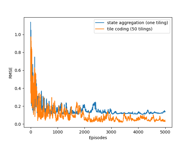
Coarse Coding

Tile Coding

Radial Basis Functions

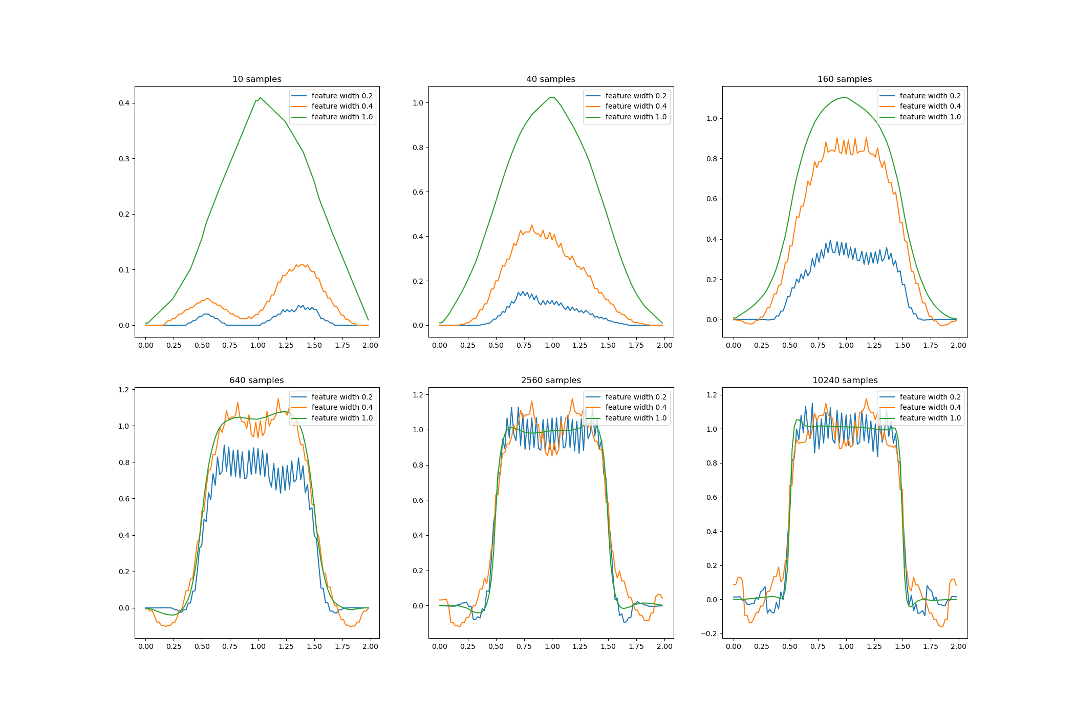
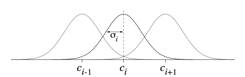
Another common scheme is Radial Basis Functions (RBFs). RBFs are the natural generalization of coarse coding to continuous valued features. Rather than each feature taking either $0$ or $1$, it can be anything within $[0,1]$, reflecting various degrees to which the feature is present.

A typical RBF feature, $x_i$, has a Gaussian response $x_i(s)$ dependent only on the distance between the state, $s$, and the feature’s prototypical or center state, $c_i$, and relative to the feature’s width, $\sigma_i$: \begin{equation} x_i(s)\doteq\exp\left(\frac{\Vert s-c_i\Vert^2}{2\sigma_i^2}\right) \end{equation} The figures below shows a one-dimensional example with a Euclidean distance metric.

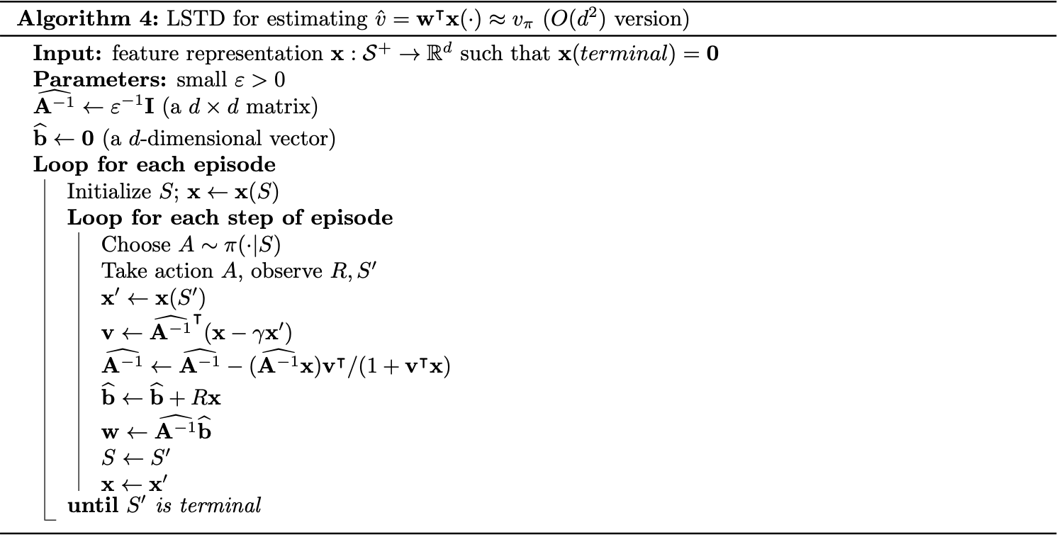
Least-Squares TD

Recall when using TD(0) with linear function approximation, $v_\mathbf{w}(s)=\mathbf{w}^\text{T}\mathbf{x}(s)$, we need to find a point $\mathbf{w}$ such that \begin{equation} \mathbb{E}\Big[\big(R_{t+1}+\gamma v_\mathbf{w}(S_{t+1})-v_{\mathbf{w}}(S_t)\big)\mathbf{x}_t\Big]=\mathbf{0}\label{eq:lstd.1} \end{equation} or \begin{equation} \mathbb{E}\Big[R_{t+1}\mathbf{x}_t-\mathbf{x}_t(\mathbf{x}_t-\gamma\mathbf{x}_{t+1})^\text{T}\mathbf{w}_t\Big]=\mathbf{0} \end{equation} We found out that the solution is: \begin{equation} \mathbf{w}_{\text{TD}}=\mathbf{A}^{-1}\mathbf{b}, \end{equation} where \begin{align} \mathbf{A}&\doteq\mathbb{E}\left[\mathbf{x}_t\left(\mathbf{x}_t-\gamma\mathbf{x}_{t+1}\right)^\text{T}\right], \\ \mathbf{b}&\doteq\mathbb{E}\left[R_{t+1}\mathbf{x}_t\right] \end{align} Instead of computing these expectations over all possible states and all possible transitions that could happen, we now only care about the things that did happen. In particular, we now consider the empirical loss of \eqref{eq:lstd.1}, as: \begin{equation} \frac{1}{t}\sum_{k=0}^{t-1}\big(R_{k+1}+\gamma v_\mathbf{w}(S_{k+1})-v_{\mathbf{w}}(S_k)\big)\mathbf{x}_i=\mathbf{0}\label{eq:lstd.2} \end{equation} By the law of large numbers³, when $t\to\infty$, \eqref{eq:lstd.2} converges to its expectation, which is \eqref{eq:lstd.1}. Hence, we now just have to compute the estimate of $\mathbf{w}_{\text{TD}}$, called $\mathbf{w}_{\text{LSTD}}$ (as LSTD stands for Least-Squares TD), which is defined as: \begin{equation} \mathbf{w}_{\text{LSTD}}\doteq\left(\sum_{k=0}^{t-1}\mathbf{x}_i\left(\mathbf{x}_k-\gamma\mathbf{x}_{k+1}\right)^\text{T}\right)^{-1}\left(\sum_{k=1}^{t-1}R_{k+1}\mathbf{x}_k\right)\label{eq:lstd.3} \end{equation} In other words, our work is to compute estimates $\widehat{\mathbf{A}}_t$ and $\widehat{\mathbf{b}}_t$ of $\mathbf{A}$ and $\mathbf{b}$: \begin{align} \widehat{\mathbf{A}}_t&\doteq\sum_{k=0}^{t-1}\mathbf{x}_k\left(\mathbf{x}_k-\gamma\mathbf{x}_{k+1}\right)^\text{T}+\varepsilon\mathbf{I};\label{eq:lstd.4} \\ \widehat{\mathbf{b}}_t&\doteq\sum_{k=0}^{t-1}R_{k+1}\mathbf{x}_k,\label{eq:lstd.5} \end{align} where $\mathbf{I}$ is the identity matrix, and $\varepsilon\mathbf{I}$, for some small $\varepsilon>0$, ensures that $\widehat{\mathbf{A}}_t$ is always invertible. Thus, \eqref{eq:lstd.3} can be rewritten as: \begin{equation} \mathbf{w}_{\text{LSTD}}\doteq\widehat{\mathbf{A}}_t^{-1}\widehat{\mathbf{b}}_t \end{equation} The two approximations in \eqref{eq:lstd.4} and \eqref{eq:lstd.5} could be implemented incrementally using the same technique we used to apply earlier so that they can be done in constant time per step. Even so, the update for $\widehat{\mathbf{A}}_t$ would have the computational complexity of $O(d^2)$, and so is its memory required to hold the $\widehat{\mathbf{A}}_t$ matrix.

This leads to a problem that our next step, which is the computation of the inverse $\widehat{\mathbf{A}}_t^{-1}$ of $\widehat{\mathbf{A}}_t$, is going to be $O(d^3)$. Fortunately, with the so-called Sherman-Morrison formula, an inverse of our special form matrix - a sum of outer products - can also be updated incrementally with only $O(d^2)$ computations, as \begin{align} \widehat{\mathbf{A}}_t^{-1}&=\left(\widehat{\mathbf{A}}_t+\mathbf{x}_t\left(\mathbf{x}_t-\gamma\mathbf{x}_{t+1}\right)^\text{T}\right)^{-1} \\ &=\widehat{\mathbf{A}}_{t-1}^{-1}-\frac{\widehat{\mathbf{A}}_{t-1}^{-1}\mathbf{x}_t\left(\mathbf{x}_t-\gamma\mathbf{x}_{t+1}\right)^\text{T}\widehat{\mathbf{A}}_{t-1}^{-1}}{1+\left(\mathbf{x}_t-\gamma\mathbf{x}_{t+1}\right)^\text{T}\widehat{\mathbf{A}}_{t-1}^{-1}\mathbf{x}_t}, \end{align} for $t>0$, with $\mathbf{\widehat{A}}_0\doteq\varepsilon\mathbf{I}$.

For the estimate $\widehat{\mathbf{b}}_t$ of $\mathbf{b}$, it can be updated using naive approach: \begin{equation} \widehat{\mathbf{b}}_{t+1}=\widehat{\mathbf{b}}_t+R_{t+1}\mathbf{x}_t \end{equation} The pseudocode for LSTD is given below

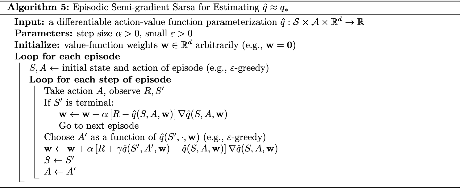
Episodic Semi-gradient Sarsa

We now consider the control problem, with parametric approximation of the action-value function $\hat{q}(s,a,\mathbf{w})\approx q_*(s,a)$, where $\mathbf{w}\in\mathbb{R}^d$ is a finite-dimensional weight vector.

Similar to the prediction problem, we can apply semi-gradient methods in solving the control problem. The difference is rather than considering training examples of the form $S_t\mapsto U_t$, we now consider examples of the form $S_t,A_t\mapsto U_t$.

From \eqref{eq:sg.2}, we can derive the general SGD update for action-value prediction as \begin{equation} \mathbf{w}_{t+1}\doteq\mathbf{w}_t+\alpha\big[U_t-\hat{q}(S_t,A_t,\mathbf{w}_t)\big]\nabla_\mathbf{w}\hat{q}(S_t,A_t,\mathbf{w}_t)\label{eq:esgs.1} \end{equation} The update for the one-step Sarsa method therefore would be \begin{equation} \mathbf{w}_{t+1}\doteq\mathbf{w}_t+\alpha\big[R_{t+1}+\gamma\hat{q}(S_{t+1},A_{t+1},\mathbf{w}_t)-\hat{q}(S_t,A_t,\mathbf{w}_t)\big]\nabla_\mathbf{w}\hat{q}(S_t,A_t,\mathbf{w}_t)\label{eq:esgs.2} \end{equation} We call this method episodic semi-gradient one-step Sarsa.

To form the control method, we need to couple the action-value

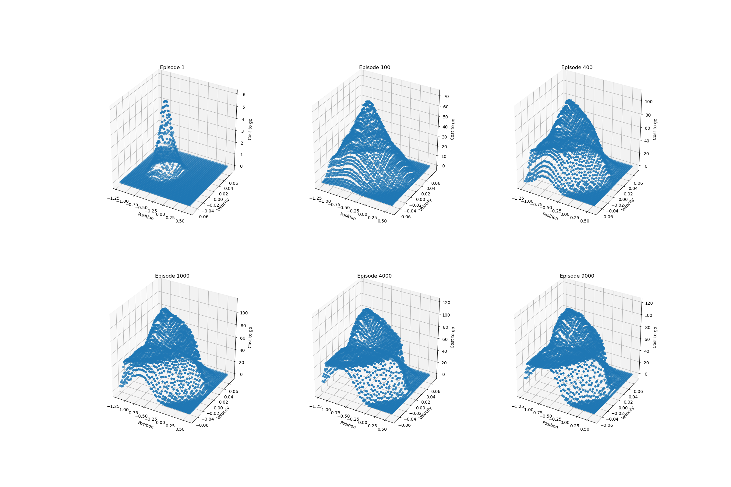
The following figure illustrates the cost-to-go function $\max_a\hat{q}(s,a,\mathbf{w})$ learned during one run of the semi-gradient Sarsa on Mountain Car task.

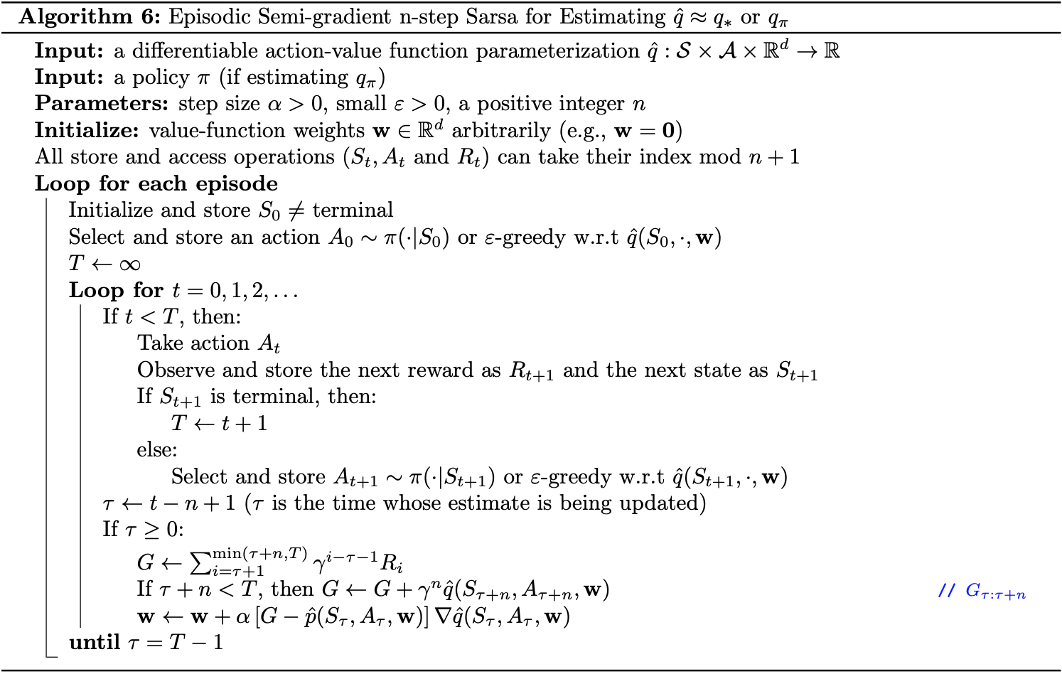
Episodic Semi-gradient $\boldsymbol{n}$-step Sarsa

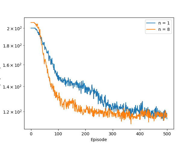
Similar to how we defined the one-step Sarsa version of semi-gradient, we can replace the update target in \eqref{eq:esgs.1} by an $n$-step return, \begin{equation} G_{t:t+n}\doteq R_{t+1}+\gamma R_{t+2}+\dots+\gamma^{n-1}R_{t+n}+\gamma^n\hat{q}(S_{t+n},A_{t+n},\mathbf{w}_{t+n-1}),\label{eq:esgnss.1} \end{equation} for $t+n\lt T$, with $G_{t:t+n}\doteq G_t$ if $t+n\geq T$, as usual, to obtain the semi-gradient $n$-step Sarsa update: \begin{equation} \mathbf{w}_{t+n}\doteq\mathbf{w}_{t+n-1}+\alpha\big[G_{t:t+n}-\hat{q}(S_t,A_t,\mathbf{w}_{t+n-1})\big]\nabla_\mathbf{w}\hat{q}(S_t,A_t,\mathbf{w}_{t+n-1}), \end{equation} for $0\leq t\lt T$. The pseudocode is given below.

The figure below shows how the $n$-step ($8$-step in particular) tends to learn faster than the one-step algorithm.

Average Reward

We now consider a new setting for continuing tasks - alongside the episodic and discounted settings - average reward.

In the average-reward setting, the quality of a policy $\pi$ is defined as the average rate of reward, or simply average reward, while following that policy, which we denote as $r(\pi)$: \begin{align} r(\pi)&\doteq\lim_{h\to\infty}\frac{1}{h}\sum_{t=1}^{h}\mathbb{E}\Big[R_t\vert S_0,A_{0:t-1}\sim\pi\Big] \\ &=\lim_{t\to\infty}\mathbb{E}\Big[R_t\vert S_0,A_{0:t-1}\sim\pi\Big] \\ &=\sum_s\mu_\pi(s)\sum_a\pi(a\vert s)\sum_{s’,r}p(s’,r\vert s,a)r, \end{align} where:

• the expectations are conditioned on the initial state $S_0$, and on the subsequent action $A_0,A_1,\dots,A_{t-1}$, being taken according to $\pi$;
• $\mu_\pi$ is the steady-state distribution, \begin{equation} \mu_\pi\doteq\lim_{t\to\infty}P\left(S_t=s\vert A_{0:t-1}\sim\pi\right), \end{equation} which is assumed to exist for any $\pi$ and to be independent of $S_0$.

The steady state distribution is the special distribution under which, if we select actions according to $\pi$, we remain in the same distribution. That is, for which \begin{equation} \sum_s\mu_\pi(x)\sum_a\pi(a\vert s)p(s’\vert s,a)=\mu_\pi(s’) \end{equation} In the average-reward setting, returns are defined in terms of differences between rewards and the average reward: \begin{equation} G_t\doteq R_{t+1}-r(\pi)+R_{t+2}-r(\pi)+R_{t+3}-r(\pi)+\dots\label{eq:ar.1} \end{equation} This is known as the differential return, and the corresponding value functions are known as differential value functions, $v_\pi(s)$ and $q_\pi(s,a)$, which are defined in the same way as we have done before: \begin{align} v_\pi(s)&\doteq\mathbb{E}\big[G_t\vert S_t=s\big]; \\ q_\pi(s,a)&\doteq\mathbb{E}\big[G_t\vert S_t=s,A_t=a\big], \end{align} and similarly for $v_{*}$ and $q_{*}$. Likewise, differential value functions also have Bellman equations, with some modifications by replacing all discounted factor $\gamma$ and replacing all rewards, $r$, by the difference between the reward and the true average reward, $r-r(\pi)$, as: \begin{align} &v_\pi(s)=\sum_a\pi(a|s)\sum_{r,s’}p(r,s’|s,a)\left[r-r(\pi)+v_\pi(s’)\right], \\ &q_\pi(s,a)=\sum_{r,s’}p(s’,r|s,a)\left[r-r(\pi)+\sum_{a’}\pi(a’|s’)q_\pi(s’,a’)\right], \\ &v_{*}(s)=\max_a\sum_{r,s’}p(s’,r|s,a)\left[r-\max_\pi r(\pi)+v_{*}(s’)\right], \\ &q_{*}(s,a)=\sum_{r,s’}p(s’,r|s,a)\left[r-\max_\pi r(\pi)+\max_{a’}q_{*}(s’,a’)\right] \end{align}

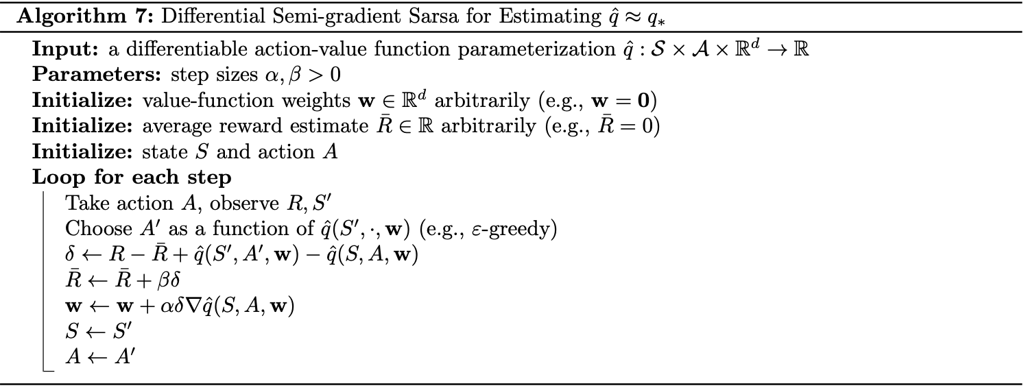
Differential Semi-gradient Sarsa

There is also a differential form of the two TD errors: \begin{equation} \delta_t\doteq R_{t+1}-\bar{R}_{t+1}+\hat{v}(S_{t+1},\mathbf{w}_t)-\hat{v}(S_t,\mathbf{w}_t), \end{equation} and \begin{equation} \delta_t\doteq R_{t+1}-\bar{R}_{t+1}+\hat{q}(S_{t+1},A_{t+1},\mathbf{w}_t)-\hat{q}(S_t,A_t,\mathbf{w}_t),\label{eq:dsgs.1} \end{equation} where $\bar{R}_t$ is an estimate at time $t$ of the average reward $r(\pi)$.

With these alternative definitions, most of our algorithms and many theoretical results carry through to the average-reward setting without change.

For example, the average reward version of semi-gradient Sarsa is defined just as in \eqref{eq:esgs.2} except with the differential version of the TD error \eqref{eq:dsgs.1}: \begin{equation} \mathbf{w}_{t+1}\doteq\mathbf{w}_t+\alpha\delta_t\nabla_\mathbf{w}\hat{q}(S_t,A_t,\mathbf{w}_t)\label{eq:dsgs.2} \end{equation} The pseudocode of the algorithm is then given below.

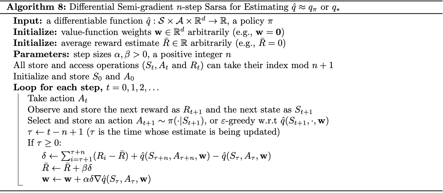
Differential Semi-gradient $\boldsymbol{n}$-step Sarsa

To derive the $n$-step version of \eqref{eq:dsgs.2}, we use the same update rule, except with an $n$-step version of the TD error.

First, we need to define the $n$-step differential return, with function approximation, by combining the idea of \eqref{eq:esgnss.1} and \eqref{eq:ar.1} together, as: \begin{equation} G_{t:t+n}\doteq R_{t+1}-\bar{R}_{t+1}+R_{t+2}-\bar{R}_{t+2}+\dots+R_{t+n}-\bar{R}_{t+n}+\hat{q}(S_{t+n},A_{t+n},\mathbf{w}_{t+n-1}), \end{equation} where $\bar{R}$ is an estimate of $r(\pi),n\geq 1$, $t+n\lt T$; $G_{t:t+n}\doteq G_t$ if $t+n\geq T$ as usual. The $n$-step TD error is then \begin{equation} \delta_t\doteq G_{t:t+n}-\hat{q}(S_t,A_t,\mathbf{w}) \end{equation} The pseudocode of the algorithm is then given below.

Off-policy Methods

We now consider off-policy methods with function approximation.

Semi-gradient

To derive the semi-gradient form of off-policy tabular methods we have known, we simply replace the update to an array ($V$ or $Q$) to an update to a weight vector $\mathbf{w}$, using the approximate value function $\hat{v}$ or $\hat{q}$ and its gradient.

Recall that in off-policy learning we seek to learn a value function for a target policy $\pi$, given data due to a different behavior policy $b$.

Many of these algorithms use the per-step importance sampling ratio: \begin{equation} \rho_t\doteq\rho_{t:t}=\dfrac{\pi(A_t|S_t)}{b(A_t|S_t)} \end{equation}

In particular, for state-value functions, the one-step algorithm is semi-gradient off-policy TD(0) has the update rule: \begin{equation} \mathbf{w}_{t+1}\doteq\mathbf{w}_t+\alpha\rho_t\delta_t\nabla_\mathbf{w}\hat{v}(S_t,\mathbf{w}_t),\label{eq:opsg.1} \end{equation} where

• If the problem is episodic and discounted, we have: \begin{equation} \delta_t\doteq R_{t+1}+\gamma\hat{v}(S_{t+1},\mathbf{w}_t)-\hat{v}(S_t,\mathbf{w}_t) \end{equation}
• If the problem is continuing and undiscounted using average reward, we have: \begin{equation} \delta_t\doteq R_{t+1}-\bar{R}+\hat{v}(S_{t+1},\mathbf{w}_t)-\hat{v}(S_t,\mathbf{w}_t) \end{equation}

For action values, the one-step algorithm is semi-gradient Expected Sarsa, which has the update rule: \begin{equation} \mathbf{w}_{t+1}\doteq\mathbf{w}_t+\alpha\delta_t\nabla_\mathbf{w}\hat{q}(S_t,A_t,\mathbf{w}), \end{equation} with

• Episodic tasks: \begin{equation} \delta_t\doteq R_{t+1}+\gamma\sum_a\pi(a\vert S_{t+1})\hat{q}(S_{t+1},a,\mathbf{w}_t)-\hat{q}(S_t,A_t,\mathbf{w}_t) \end{equation}
• Continuing tasks: \begin{equation} \delta_t\doteq R_{t+1}-\bar{R}+\sum_a\pi(a\vert S_{t+1})\hat{q}(S_{t+1},a,\mathbf{w}_t)-\hat{q}(S_t,A_t,\mathbf{w}_t) \end{equation}

With multi-step algorithms, we begin with semi-gradient $\boldsymbol{n}$-step Expected Sarsa, which has the update rule: \begin{equation} \hspace{-0.8cm}\mathbf{w}_{t+n}\doteq\mathbf{w}_{t+n-1}+\alpha\rho_{t+1}\dots\rho_{t+n-1}\big[G_{t:t+n}-\hat{q}(S_t,A_t,\mathbf{w}_{t+n-1})\big]\nabla_\mathbf{w}\hat{q}(S_t,A_t,\mathbf{w}_{t+n-1}), \end{equation} where $\rho_k=1$ for $k\geq T$ and $G_{t:n}\doteq G_t$ if $t+n\geq T$, and with

• Episodic tasks: \begin{equation} G_{t:t+n}\doteq R_{t+1}+\dots+\gamma^{n-1}R_{t+n}+\gamma^n\hat{q}(S_{t+n},A_{t+n},\mathbf{w}_{t+n-1}) \end{equation}
• Continuing tasks: \begin{equation} G_{t:t+n}\doteq R_{t+1}-\bar{R}_t+\dots+R_{t+n}-\bar{R}_{t+n-1}+\hat{q}(S_{t+n},A_{t+n},\mathbf{w}_{t+n-1}), \end{equation}

For the semi-gradient version of $n$-step tree-backup, called semi-gradient $\boldsymbol{n}$-step tree-backup, the update rule is: \begin{equation} \mathbf{w}_{t+n}\doteq\mathbf{w}_{t+n-1}+\alpha\big[G_{t:t+n}-\hat{q}(S_t,A_t,\mathbf{w}_{t+n-1})\big]\nabla_\mathbf{w}\hat{q}(S_t,A_t,\mathbf{w}_{t+n-1}), \end{equation} where \begin{equation} G_{t:t+n}\doteq\hat{q}(S_t,A_t,\mathbf{w}_{t-1})+\sum_{k=t}^{t+n-1}\delta_k\prod_{i=t+1}^{k}\gamma\pi(A_i|S_i), \end{equation} with $\delta_t$ is defined similar to the case of semi-gradient Expected Sarsa.

Residual Bellman Update

Gradient-TD

In this section, we will be considering SGD methods for minimizing the $\overline{\text{PBE}}$.

Rewrite the objective $\overline{\text{PBE}}$ in matrix terms, we have: \begin{align} \overline{\text{PBE}}(\mathbf{w})&=\left\Vert\Pi\bar{\delta}_\mathbf{w}\right\Vert_{\mu}^{2} \\ &=\left(\Pi\bar{\delta}_\mathbf{w}\right)^\text{T}\mathbf{D}\Pi\bar{\delta}_\mathbf{w} \\ &=\bar{\delta}_\mathbf{w}^\text{T}\Pi^\text{T}\mathbf{D}\Pi\bar{\delta}_\mathbf{w} \\ &=\bar{\delta}_\mathbf{w}^\text{T}\mathbf{D}\mathbf{X}\left(\mathbf{X}^\text{T}\mathbf{D}\mathbf{X}\right)^{-1}\mathbf{X}^\text{T}\mathbf{D}\bar{\delta}_\mathbf{w} \\ &=\left(\mathbf{X}^\text{T}\mathbf{D}\bar{\delta}_\mathbf{w}\right)^\text{T}\left(\mathbf{X}^\text{T}\mathbf{D}\mathbf{X}\right)^{-1}\left(\mathbf{X}^\text{T}\mathbf{D}\bar{\delta}_\mathbf{w}\right), \end{align} where in the fourth step, we use the property of projection operation⁴ and the identity \begin{equation} \Pi^\text{T}\mathbf{D}\Pi=\mathbf{D}\mathbf{X}\left(\mathbf{X}^\text{T}\mathbf{D}\mathbf{X}\right)^{-1}\mathbf{X}^\text{T}\mathbf{D} \end{equation} Thus, the gradient w.r.t weight vector $\mathbf{w}$ is \begin{equation} \nabla_\mathbf{w}\overline{\text{PBE}}(\mathbf{w})=2\nabla_\mathbf{w}\left[\mathbf{X}^\text{T}\mathbf{D}\bar{\delta}_\mathbf{w}\right]^\text{T}\left(\mathbf{X}^\text{T}\mathbf{D}\mathbf{X}\right)^{-1}\left(\mathbf{X}^\text{T}\mathbf{D}\bar{\delta}_\mathbf{w}\right)\label{eq:gt.1} \end{equation}

To turn this into an SGD method, we have to sample something on every time step that has this gradient as its expected value. Let $\mu$ be the distribution of states visited under the behavior policy. The last factor of \eqref{eq:gt.1} can be written as: \begin{equation} \mathbf{X}^\text{T}\mathbf{D}\bar{\delta}_\mathbf{w}=\sum_s\mu(s)\mathbf{x}(s)\bar{\delta}_\mathbf{w}=\mathbb{E}\left[\rho_t\delta_t\mathbf{x}_t\right], \end{equation} which is the expectation of the semi-gradient TD(0) update \eqref{eq:opsg.1}. The first factor of \eqref{eq:gt.1}, which is the transpose of the gradient of this update, then can also be written as: \begin{align} \nabla_\mathbf{w}\mathbb{E}\left[\rho_t\delta_t\mathbf{x}_t\right]^\text{T}&=\mathbb{E}\left[\rho_t\nabla_\mathbf{w}\delta_t^\text{T}\mathbf{x}_t^\text{T}\right] \\ &=\mathbb{E}\left[\rho_t\nabla_\mathbf{w}\left(R_{t+1}+\gamma\mathbf{w}^\text{T}\mathbf{x}_{t+1}-\mathbf{w}^\text{T}\mathbf{x}_t\right)^\text{T}\mathbf{x}_t^\text{T}\right] \\ &=\mathbb{E}\left[\rho_t\left(\gamma\mathbf{x}_{t+1}-\mathbf{x}_t\right)\mathbf{x}_t^\text{T}\right] \end{align} And the middle factor, without the inverse operation, can also be written as: \begin{equation} \mathbf{X}^\text{T}\mathbf{D}\mathbf{X}=\sum_a\mu(s)\mathbf{x}_s\mathbf{x}_s^\text{T}=\mathbb{E}\left[\mathbf{x}_t\mathbf{x}_t^\text{T}\right] \end{equation} Substituting these expectations back to \eqref{eq:gt.1}, we obtain: \begin{equation} \nabla_\mathbf{w}\overline{\text{PBE}}(\mathbf{w})=2\mathbb{E}\left[\rho_t\left(\gamma\mathbf{x}_{t+1}-\mathbf{x}_t\right)\mathbf{x}_t^\text{T}\right]\mathbb{E}\left[\mathbf{x}_t\mathbf{x}_t^\text{T}\right]^{-1}\mathbb{E}\left[\rho_t\delta_t\mathbf{x}_t\right]\label{eq:gt.2} \end{equation}

Here, we use the Gradient-TD to estimate and store the product of the second two factors in \eqref{eq:gt.2}, denoted as $\mathbf{v}$: \begin{equation} \mathbf{v}\approx\mathbb{E}\left[\mathbf{x}_t\mathbf{x}_t^\text{T}\right]^{-1}\mathbb{E}\left[\rho_t\delta_t\mathbf{x}_t\right],\label{eq:gt.3} \end{equation} which is the solution of the linear least-squares problem that tries to approximate $\rho_t\delta_t$ from the features. The SGD for incrementally finding the vector $\mathbf{v}$ that minimizes the expected squared error $\left(\mathbf{v}^\text{T}\mathbf{x}_t\right)^2$ is known as the Least Mean Square (LMS) rule (here augmented with an IS ratio): \begin{equation} \mathbf{v}_{t+1}\doteq\mathbf{v}_t+\beta\rho_t\left(\delta_t-\mathbf{v}^\text{T}\mathbf{x}_t\right)\mathbf{x}_t, \end{equation} where $\beta>0$ is a step-size parameter.

With a given stored estimate $\mathbf{v}_t$ approximating \eqref{eq:gt.3}, we can apply SGD update to the parameter $\mathbf{w}_t$: \begin{align} \mathbf{w}_{t+1}&=\mathbf{w}_t-\frac{1}{2}\alpha\nabla_\mathbf{w}\overline{\text{PBE}}(\mathbf{w}_t) \\ &=\mathbf{w}_t-\frac{1}{2}\alpha 2\mathbb{E}\left[\rho_t\left(\gamma\mathbf{x}_{t+1}-\mathbf{x}_t\right)\mathbf{x}_t^\text{T}\right]\mathbb{E}\left[\mathbf{x}_t\mathbf{x}_t^\text{T}\right]^{-1}\mathbb{E}\left[\rho_t\delta_t\mathbf{x}_t\right] \\ &=\mathbf{w}_t+\alpha\mathbb{E}\left[\rho_t\left(\mathbf{x}_t-\gamma\mathbf{x}_{t+1}\right)\mathbf{x}_t^\text{T}\right]\mathbb{E}\left[\mathbf{x}_t\mathbf{x}_t^\text{T}\right]^{-1}\mathbb{E}\left[\rho_t\delta_t\mathbf{x}_t\right]\label{eq:gt.4} \\ &\approx\mathbf{w}_t+\alpha\mathbb{E}\left[\rho_t\left(\mathbf{x}_t-\gamma\mathbf{x}_{t+1}\right)\mathbf{x}_t^\text{T}\right]\mathbf{v}_t \\ &\approx\mathbf{w}_t+\alpha\rho_t\left(\mathbf{x}_t-\gamma\mathbf{x}_{t+1}\right)\mathbf{x}_t\mathbf{v}_t \end{align} This algorithm is called GTD2. From \eqref{eq:gt.4}, we can also continue to derive as: \begin{align} \mathbf{w}_{t+1}&=\mathbf{w}_t+\alpha\mathbb{E}\left[\rho_t\left(\mathbf{x}_t-\gamma\mathbf{x}_{t+1}\right)\mathbf{x}_t^\text{T}\right]\mathbb{E}\left[\mathbf{x}_t\mathbf{x}_t^\text{T}\right]^{-1}\mathbb{E}\left[\rho_t\delta_t\mathbf{x}_t\right] \\ &=\mathbf{w}_t+\alpha\left(\mathbb{E}\left[\rho_t\mathbf{x}_t\mathbf{x}_t^\text{T}\right]-\gamma\mathbb{E}\left[\rho_t\mathbf{x}_{t+1}\mathbf{x}_t^\text{T}\right]\right)\mathbb{E}\left[\mathbf{x}_t\mathbf{x}_t^\text{T}\right]^{-1}\mathbb{E}\left[\rho_t\delta_t\mathbf{x}_t\right] \\ &=\mathbf{w}_t+\alpha\left(\mathbb{E}\left[\mathbf{x}_t\mathbf{x}_t^\text{T}\right]-\gamma\mathbb{E}\left[\rho_t\mathbf{x}_{t+1}\mathbf{x}_t^\text{T}\right]\right)\mathbb{E}\left[\mathbf{x}_t\mathbf{x}_t^\text{T}\right]^{-1}\mathbb{E}\left[\rho_t\delta_t\mathbf{x}_t\right] \\ &=\mathbf{w}_t+\alpha\left(\mathbb{E}\left[\mathbf{x}_t\rho_t\delta_t\right]-\gamma\mathbb{E}\left[\rho_t\mathbf{x}_{t+1}\mathbf{x}_t^\text{T}\right]\mathbb{E}\left[\mathbf{x}_t\mathbf{x}_t^\text{T}\right]^{-1}\mathbb{E}\left[\rho_t\delta_t\mathbf{x}_t\right]\right) \\ &\approx\mathbf{w}_t+\alpha\left(\mathbb{E}\left[\mathbf{x}_t\rho_t\delta_t\right]-\gamma\mathbb{E}\left[\rho_t\mathbf{x}_{t+1}\mathbf{x}_t^\text{T}\right]\right)\mathbf{v}_t \\ &\approx\mathbf{w}_t+\alpha\rho_t\left(\delta_t\mathbf{x}_t-\gamma\mathbf{x}_{t+1}\mathbf{x}_t^\text{T}\mathbf{v}_t\right) \end{align} This algorithm is known as TD(0) with gradient correction (TDC), or as GTD(0).

Emphatic-TD

References

[1] Richard S. Sutton & Andrew G. Barto. Reinforcement Learning: An Introduction. MIT press, 2018.

[2] Deepmind x UCL. Reinforcement Learning Lecture Series 2021.

[3] Richard S. Sutton. Learning to predict by the methods of temporal differences. Machine Learning, 3, 9–44, 1988.

[4] Konidaris, G. & Osentoski, S. & Thomas, P.. Value Function Approximation in Reinforcement Learning Using the Fourier Basis. AAAI Conference on Artificial Intelligence, North America, aug. 2011.

[5] Joseph K. Blitzstein & Jessica Hwang. Introduction to Probability.

[6] Shangtong Zhang. Reinforcement Learning: An Introduction implementation. Github.

Footnotes