Eligible Traces

Beside $n$-step TD methods, there is another mechanism called eligible traces that unify TD and Monte Carlo. Setting $\lambda$ in TD($\lambda$) from $0$ to $1$, we end up with a spectrum ranging from TD methods, when $\lambda=0$ to Monte Carlo methods with $\lambda=1$.

The $\lambda$-return

Recall that in TD-Learning note, we have defined the $n$-step return as \begin{equation} G_{t:t+n}\doteq R_{t+1}+\gamma R_{t+2}+\dots+\gamma^{n-1}R_{t+n}V_{t+n-1}(S_{t+n}) \end{equation} for all $n,t$ such that $n\geq 1$ and $0\leq t\lt T-n$. After the note of Function Approximation, for any parameterized function approximator, we can generalize that equation into: \begin{equation} G_{t:t+n}\doteq R_{t+1}+\gamma R_{t+2}+ \dots+\gamma^{n-1}R_{t+n}+\gamma^n\hat{v}(S_{t+n},\mathbf{w}_{t+n-1}),\hspace{1cm}0\leq t\leq T-n \end{equation} where $\hat{v}(s,\mathbf{w})$ is the approximate value of state $s$ given weight vector $\mathbf{w}$.

We already know that by selecting $n$-step return as the target for a tabular learning update, just as it is for an approximate SGD update, we can reach to an optimal point. In fact, a valid update can be also be done toward any average of $n$-step returns for different $n$. For example, we can choose \begin{equation} \frac{1}{2}G_{t:t+2}+\frac{1}{2}G_{t:t+4} \end{equation} as the target for our update.

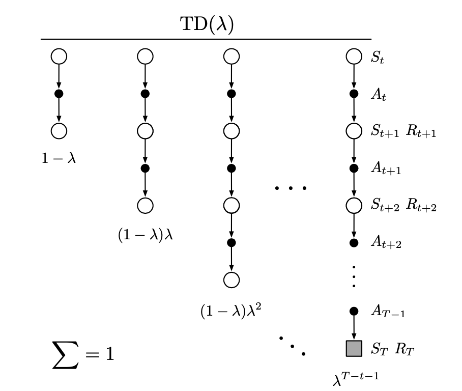
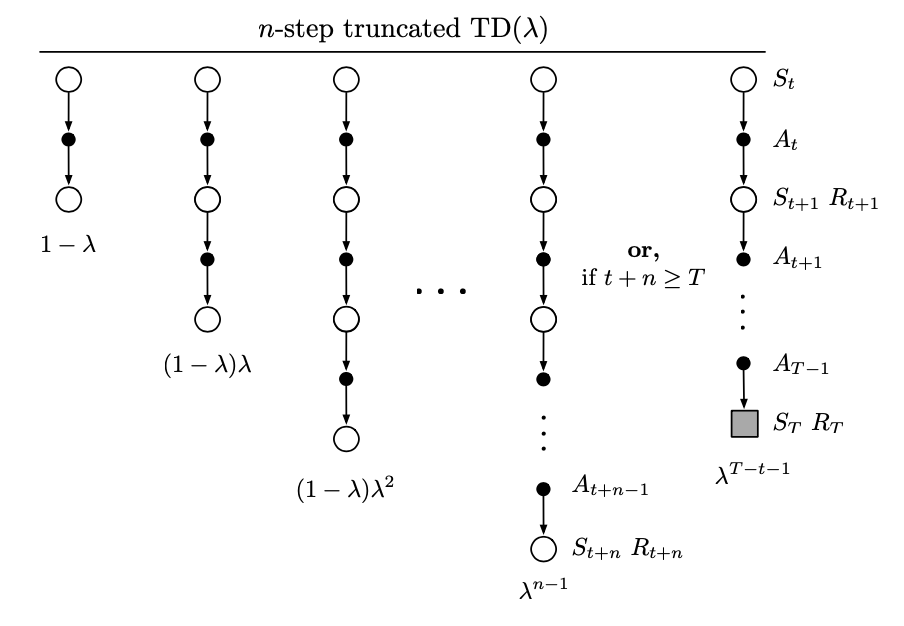
The TD($\lambda$) is a particular way of averaging $n$-step updates. This average contains all the $n$-step updates, each weighted proportionally to $\lambda^{n-1}$, for $\lambda\in\left[0,1\right]$, and is normalized by a factor of $1-\lambda$ to guarantee that the weights sum to $1$, as: \begin{equation} G_t^\lambda\doteq(1-\lambda)\sum_{n=1}^{\infty}\lambda^{n-1}G_{t:t+n} \end{equation} The $G_t^\lambda$ is called $\lambda$-return of the update.

This figure below illustrates the backup diagram of TD($\lambda$) algorithm.

Offline $\lambda$-return

With the definition of $\lambda$-return, we can define the offline $\lambda$-return algorithm, which use semi-gradient update and using $\lambda$-return as the target: \begin{equation} \mathbf{w}_{t+1}\doteq\mathbf{w}_t+\alpha\left[G_t^\lambda-\hat{v}(S_t,\mathbf{w}_t)\right]\nabla_\mathbf{w}\hat{v}(S_t,\mathbf{w}_t),\hspace{1cm}t=0,\dots,T-1 \end{equation}

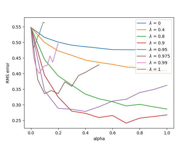
A result when applying offline $\lambda$-return on the random walk problem is shown below.

TD($\lambda$)

TD($\lambda$) improves over the offline $\lambda$-return algorithm since:

• It updates the weight vector $\mathbf{w}$ on every step of an episode rather than only at the end, which leads to a time improvement.
• Its computations are equally distributed in time rather than all at the end of the episode.
• It can be applied to continuing problems rather than just to episodic ones.

With function approximation, the eligible trace is a vector $\mathbf{z}_t\in\mathbb{R}^d$ with the same number of components as the weight vector $\mathbf{w}_t$. Whereas $\mathbf{w}_t$ is long-term memory, $\mathbf{z}_t$ on the other hand is a short-term memory, typically lasting less time than the length of an episode.

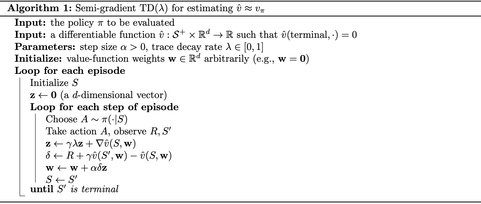
In TD($\lambda$), starting at the initial value of zero at the beginning of the episode, on each time step, the eligible trace vector $\mathbf{z}_t$ is incremented by the value gradient, and then fades away by $\gamma\lambda$: \begin{align} \mathbf{z}_{-1}&\doteq\mathbf{0} \\ \mathbf{z}_t&\doteq\gamma\lambda\mathbf{z}_{t-1}+\nabla_\mathbf{w}\hat{v}(S_t,\mathbf{w}_t),\hspace{1cm}0\leq t\lt T\label{eq:tl.1} \end{align} where $\gamma$ is the discount factor; $\lambda$ is also called trace-decay parameter. On the other hand, the weight vector $\mathbf{w}_t$ is updated on each step proportional to the scalar TD errors and the eligible trace vector $\mathbf{z}_t$: \begin{equation} \mathbf{w}_{t+1}\doteq\mathbf{w}_t+\alpha\delta_t\mathbf{z}_t,\label{eq:tl.2} \end{equation} where the TD error is defined as \begin{equation} \delta_t\doteq R_{t+1}+\gamma\hat{v}(S_{t+1},\mathbf{w}_t)-\hat{v}(S_t,\mathbf{w}_t) \end{equation} Pseudocode of semi-gradient TD($\lambda$) is given below.

Linear TD($\lambda$) has been proved to converge in the on-policy case if the step size parameter, $\alpha$, is reduced over time according to the usual conditions. And also in the continuing discounted case, for any $\lambda$, $\overline{\text{VE}}$ is proven to be within a bounded expansion of the lowest possible error: \begin{equation} \overline{\text{VE}}(\mathbf{w}_\infty)\leq\dfrac{1-\gamma\lambda}{1-\gamma}\min_\mathbf{w}\overline{\text{VE}}(\mathbf{w}) \end{equation}

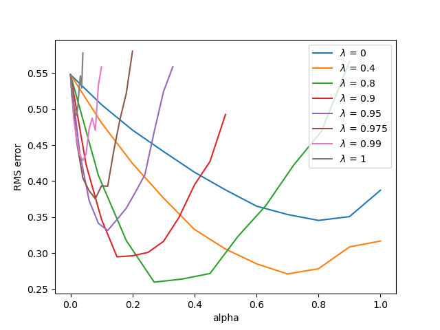
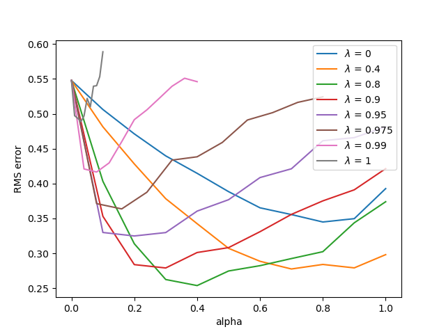
The figure below illustrates the result for using TD($\lambda$) on the usual random walk task.

Truncated TD Methods

Since in the offline $\lambda$-return, the target $\lambda$-return is not known until the end of episode. And moreover, in the continuing case, since the $n$-step returns depend on arbitrary large $n$, it maybe never known. However, the dependence becomes weaker for longer-delayed rewards, falling by $\gamma\lambda$ for each step of delay.

A natural approximation is to truncate the sequence after some number of steps. In general, we define the truncated $\lambda$-return for time $t$, given data only up to some later horizon, $h$, as: \begin{equation} G_{t:h}^\lambda\doteq(1-\lambda)\sum_{n=1}^{h-t-1}\lambda^{n-1}G_{t:t+n}+\lambda^{h-t-1}G_{t:h},\hspace{1cm}0\leq t\lt h\leq T \end{equation} With this definition of the return, and based on the function approximation version of the $n$-step TD we have defined before, we have the TTD($\lambda$) is defined as: \begin{equation} \mathbf{w}_{t+n}\doteq\mathbf{w}_{t+n-1}+\alpha\left[G_{t:t+n}^\lambda-\hat{v}(S_t,\mathbf{w}_{t+n-1})\right]\nabla_\mathbf{w}\hat{w}(S_t,\mathbf{w}_{t+n-1}),\hspace{1cm}0\leq t\lt T \end{equation} We have the $k$-step $\lambda$-return can be written as: \begin{align} \hspace{-0.8cm}G_{t:t+k}^\lambda&=(1-\lambda)\sum_{n=1}^{k-1}\lambda^{n-1}G_{t:t+n}+\lambda^{k-1}G_{t:t+k} \\ &=(1-\lambda)\sum_{n=1}^{k-1}\lambda^{n-1}\left[R_{t+1}+\gamma R_{t+2}+\dots+\gamma^{n-1}R_{t+n}+\gamma^n\hat{v}(S_{t+n},\mathbf{w}_{t+n-1})\right]\nonumber \\ &\hspace{1cm}+\lambda^{k-1}\left[R_{t+1}+\gamma R_{t+2}+\dots+\gamma^{k-1}R_{t+k}+\gamma^k\hat{v}(S_{t+k},\mathbf{w}_{t+k-1})\right] \\ &=R_{t+1}+\gamma\lambda R_{t+2}+\dots+\gamma^{k-1}\lambda^{k-1}R_{t+k}\nonumber \\ &\hspace{1cm}+(1-\lambda)\left[\sum_{n=1}^{k-1}\lambda^{n-1}\gamma^n\hat{v}(S_{t+n},\mathbf{w}_{t+n-1})\right]+\lambda^{k-1}\gamma^k\hat{v}(S_{t+k},\mathbf{w}_{t+k-1}) \\ &=\hat{v}(S_t,\mathbf{w}_{t-1})+\left[R_{t+1}+\gamma\hat{v}(S_{t+1},\mathbf{w}_t)-\hat{v}(S_t,\mathbf{w}_{t-1})\right]\nonumber \\ &\hspace{1cm}+\left[\lambda\gamma R_{t+2}+\lambda\gamma^2\hat{v}(S_{t+2},\mathbf{w}_{t+1})-\lambda\gamma\hat{v}(S_{t+1},\mathbf{w}_t)\right]+\dots\nonumber \\ &\hspace{1cm}+\left[\lambda^{k-1}\gamma^{k-1}R_{t+k}+\lambda^{k-1}\gamma^k\hat{v}(S_{t+k},\mathbf{w}_{t+k-1})-\lambda^{k-1}\gamma^{k-1}\hat{v}(S_{t+k-1},\mathbf{w}_{t+k-2})\right] \\ &=\hat{v}(S_t,\mathbf{w}_{t-1})+\sum_{i=t}^{t+k-1}(\gamma\lambda)^{i-t}\delta_i’,\label{eq:tt.1} \end{align} with \begin{equation} \delta_t’\doteq R_{t+1}+\gamma\hat{v}(S_{t+1},\mathbf{w}_t)-\hat{v}(S_t,\mathbf{w}_{t-1}), \end{equation} where in the third step of the derivation, we use the identity \begin{equation} (1-\lambda)(1+\lambda+\dots+\lambda^{k-2})=1-\lambda^{k-1} \end{equation} From \eqref{eq:tt.1}, we can see that the $k$-step $\lambda$-return can be written as sums of TD errors if the value function is held constant, which allows us to implement the TTD($\lambda$) algorithm efficiently.

Online $\lambda$-return

The idea of online $\lambda$-return involves multiple passes over the episode, one at each horizon, each generating a different sequence of weight vectors.

Let $\mathbf{w}_t^h$ denote the weights used to generate the value at time $t$ in the sequence up to horizon $h$. The first weight vector $\mathbf{w}_0^h$ in each sequence is the one that inherited from the previous episode (thus they are the same for all $h$), and the last weight vector $\mathbf{w}_h^h$ in each sequence defines the weight-vector sequence of the algorithm. At the final horizon $h=T$, we obtain the final weight $\mathbf{w}_T^T$ which will be passed on to form the initial weights of the next episode.

In particular, we can define the first three sequences as: \begin{align} h=1:\hspace{1cm}&\mathbf{w}_1^1\doteq\mathbf{w}_0^1+\alpha\left[G_{0:1}^\lambda-\hat{v}(S_0,\mathbf{w}_0^1)\right]\nabla_\mathbf{w}\hat{v}(S_0,\mathbf{w}_0^1), \\\nonumber \\ h=2:\hspace{1cm}&\mathbf{w}_1^2\doteq\mathbf{w}_0^2+\alpha\left[G_{0:2}^\lambda-\hat{v}(S_0,\mathbf{w}_0^2)\right]\nabla_\mathbf{w}\hat{v}(S_0,\mathbf{w}_0^2), \\ &\mathbf{w}_2^2\doteq\mathbf{w}_1^2+\alpha\left[G_{1:2}^\lambda-\hat{v}(S_t,\mathbf{w}_1^2)\right]\nabla_\mathbf{w}\hat{v}(S_1,\mathbf{w}_1^2), \\\nonumber \\ h=3:\hspace{1cm}&\mathbf{w}_1^3\doteq\mathbf{w}_0^3+\alpha\left[G_{0:3}^\lambda-\hat{v}(S_0,\mathbf{w}_0^3)\right]\nabla_\mathbf{w}\hat{v}(S_0,\mathbf{w}_0^3), \\ &\mathbf{w}_2^3\doteq\mathbf{w}_1^3+\alpha\left[G_{1:3}^\lambda-\hat{v}(S_1,\mathbf{w}_1^3)\right]\nabla_\mathbf{w}\hat{v}(S_1,\mathbf{w}_1^3), \\ &\mathbf{w}_3^3\doteq\mathbf{w}_2^3+\alpha\left[G_{2:3}^\lambda-\hat{v}(S_2,\mathbf{w}_2^3)\right]\nabla_\mathbf{w}\hat{v}(S_2,\mathbf{w}_2^3) \end{align} The general form for the update of the online $\lambda$-return is \begin{equation} \mathbf{w}_{t+1}^h\doteq\mathbf{w}_t^h+\alpha\left[G_{t:h}^\lambda-\hat{v}(S_t,\mathbf{w}_t^h)\right]\nabla_\mathbf{w}\hat{v}(S_t,\mathbf{w}_t^h),\hspace{1cm}0\leq t\lt h\leq T,\label{eq:olr.1} \end{equation} with $\mathbf{w}_t\doteq\mathbf{w}_t^t$, and $\mathbf{w}_0^h$ is the same for all $h$, we denote this vector as $\mathbf{w}_{init}$.

The online $\lambda$-return algorithm is fully online, determining a new weight vector $\mathbf{w}_t$ at each time step $t$ during an episode, using only information available at time $t$. Whereas the offline version passes through all the steps at the time of termination but does not make any updates during the episode.

True Online TD($\lambda$)

In the online $\lambda$-return, at each time step a sequence of updates is performed. The length of this sequence, and hence the computation per time step, increase over time.

However, it is possible to compute the weight vector resulting from time step $t+1$, $\mathbf{w}_{t+1}$, directly from the weight vector resulting from the sequence at time step $t$, $\mathbf{w}_t$.

Consider using linear approximation for our task, which gives us \begin{align} \hat{v}(S_t,\mathbf{w}_t)&=\mathbf{w}_t^\text{T}\mathbf{x}_t; \\ \nabla_\mathbf{w}\hat{v}(S_t,\mathbf{w}_t)&=\mathbf{x}_t, \end{align} where $\mathbf{x}_t=\mathbf{x}(S_t)$ as usual.

We begin by rewriting \eqref{eq:olr.1}, as \begin{align} \mathbf{w}_{t+1}^h&\doteq\mathbf{w}_t^h+\alpha\left[G_{t:h}^\lambda-\hat{v}(S_t,\mathbf{w}_t^h)\right]\nabla_\mathbf{w}\hat{v}(S_t,\mathbf{w}_t^h) \\ &=\mathbf{w}_t^h+\alpha\left[G_{t:h}^\lambda-\left(\mathbf{w}_t^h\right)^\text{T}\mathbf{x}_t\right]\mathbf{x}_t \\ &=\left(\mathbf{I}-\alpha\mathbf{x}_t\mathbf{x}_t^\text{T}\right)\mathbf{w}_t^h+\alpha\mathbf{x}_t G_{t:h}^\lambda, \end{align} where $\mathbf{I}$ is the identity matrix. With this equation, consider $\mathbf{w}_t^h$ in the cases of $t=1$ and $t=2$, we have: \begin{align} \mathbf{w}_1^h&=\left(\mathbf{I}-\alpha\mathbf{x}_0\mathbf{x}_0^\text{T}\right)\mathbf{w}_0^h+\alpha\mathbf{x}_0 G_{0:h}^\lambda \\ &=\left(\mathbf{I}-\alpha\mathbf{x}_0\mathbf{x}_0^\text{T}\right)\mathbf{w}_{init}+\alpha\mathbf{x}_0 G_{0:h}^\lambda, \\ \mathbf{w}_2^h&=\left(\mathbf{I}-\alpha\mathbf{x}_1\mathbf{x}_1^\text{T}\right)\mathbf{w}_1^h+\alpha\mathbf{x}_1 G_{1:h}^\lambda \\ &=\left(\mathbf{I}-\alpha\mathbf{x}_1\mathbf{x}_1^\text{T}\right)\left(\mathbf{I}-\alpha\mathbf{x}_0\mathbf{x}_0^\text{T}\right)\mathbf{w}_{init}+\alpha\left(\mathbf{I}-\alpha\mathbf{x}_1\mathbf{x}_1^\text{T}\right)\mathbf{x}_0 G_{0:h}^\lambda+\alpha\mathbf{x}_1 G_{1:h}^\lambda \end{align} In general, for $t\leq h$, we can write: \begin{equation} \mathbf{w}_t^h=\mathbf{A}_0^{t-1}\mathbf{w}_{init}+\alpha\sum_{i=0}^{t-1}\mathbf{A}_{i+1}^{t-1}\mathbf{x}_i G_{i:h}^\lambda, \end{equation} where $\mathbf{A}_i^j$ is defined as: \begin{equation} \mathbf{A}_i^j\doteq\left(\mathbf{I}-\alpha\mathbf{x}_j\mathbf{x}_j^\text{T}\right)\left(\mathbf{I}-\alpha\mathbf{x}_{j-1}\mathbf{x}_{j-1}^\text{T}\right)\dots\left(\mathbf{I}-\alpha\mathbf{x}_i\mathbf{x}_i^\text{T}\right),\hspace{1cm}j\geq i, \end{equation} with $\mathbf{A}_{j+1}^j\doteq\mathbf{I}$. Hence, we can express $\mathbf{w}_t$ as: \begin{equation} \mathbf{w}_t=\mathbf{w}_t^t=\mathbf{A}_0^{t-1}\mathbf{w}_{init}+\alpha\sum_{i=0}^{t-1}\mathbf{A}_{i+1}^{t-1}\mathbf{x}_i G_{i:t}^\lambda\label{eq:totl.1} \end{equation} Using \eqref{eq:tt.1}, we have: \begin{align} G_{i:t+1}^\lambda-G_{i:t}^\lambda&=\mathbf{w}_i^\text{T}\mathbf{x}_i+\sum_{j=1}^{t}(\gamma\lambda)^{j-i}\delta_j’-\left(\mathbf{w}_i^\text{T}\mathbf{x}_i+\sum_{j=1}^{t-1}(\gamma\lambda)^{j-i}\delta_j’\right) \\ &=(\gamma\lambda)^{t-i}\delta_t’\label{eq:totl.2} \end{align} with the TD error, $\delta_t’$ is defined as earlier: \begin{equation} \delta_t’\doteq R_{t+1}+\gamma\mathbf{w}_t^\text{T}\mathbf{x}_{t+1}-\mathbf{w}_{t-1}^\text{T}\mathbf{x}_t\label{eq:totl.3} \end{equation} Using \eqref{eq:totl.1}, \eqref{eq:totl.2} and \eqref{eq:totl.3}, we have: \begin{align} \mathbf{w}_{t+1}&=\mathbf{A}_0^t\mathbf{w}_{init}+\alpha\sum_{i=0}^{t}\mathbf{A}_{i+1}^t\mathbf{x}_i G_{i:t+1}^\lambda \\ &=\mathbf{A}_0^t\mathbf{w}_{init}+\alpha\sum_{i=0}^{t-1}\mathbf{A}_{i+1}^t\mathbf{x}_i G_{i:t+1}^\lambda+\alpha\mathbf{x}_t G_{t:t+1}^\lambda \\ &=\mathbf{A}_0^t\mathbf{w}_0+\alpha\sum_{i=0}^{t-1}\mathbf{A}_{i+1}^t\mathbf{x}_i G_{i:t}^\lambda+\alpha\sum_{i=0}^{t-1}\mathbf{A}_{i+1}^t\mathbf{x}_i\left(G_{i:t+1}^\lambda-G_{i:t}^\lambda\right)+\alpha\mathbf{x}_t G_{t:t+1}^\lambda \\ &=\left(\mathbf{I}-\alpha\mathbf{x}_t\mathbf{x}_t^\text{T}\right)\left(\mathbf{A}_0^{t-1}\mathbf{w}_0+\alpha\sum_{i=0}^{t-1}\mathbf{A}_{i+1}^{t-1}\mathbf{x}_i G_{t:t+1}^\lambda\right)\nonumber \\ &\hspace{1cm}+\alpha\sum_{i=0}^{t-1}\mathbf{A}_{i+1}^t\mathbf{x}_i\left(G_{i:t+1}^\lambda-G_{i:t}^\lambda\right)+\alpha\mathbf{x}_t G_{t:t+1}^\lambda \\ &=\left(\mathbf{I}-\alpha\mathbf{x}_t\mathbf{x}_t^\text{T}\right)\mathbf{w}_t+\alpha\sum_{i=0}^{t-1}\mathbf{A}_{i+1}^t\mathbf{x}_i\left(G_{i:t+1}^\lambda-G_{i:t}^\lambda\right)+\alpha\mathbf{x}_t G_{t:t+1}^\lambda \\ &=\left(\mathbf{I}-\alpha\mathbf{x}_t\mathbf{x}_t^\text{T}\right)\mathbf{w}_t+\alpha\sum_{i=0}^{t-1}\mathbf{A}_{i+1}^t\mathbf{x}_i(\gamma\lambda)^{t-i}\delta_t’+\alpha\mathbf{x}_t\left(R_{t+1}+\gamma\mathbf{w}_t^\text{T}\mathbf{x}_{t+1}\right) \\ &=\mathbf{w}_t+\alpha\sum_{i=0}^{t-1}\mathbf{A}_{i+1}^t\mathbf{x}_t(\gamma\lambda)^{t-i}\delta_t’+\alpha\mathbf{x}_t\left(R_{t+1}+\gamma\mathbf{w}_t^\text{T}\mathbf{x}_{t+1}-\mathbf{w}_t\mathbf{x}_t\right) \\ &=\mathbf{w}_t+\alpha\sum_{i=0}^{t-1}\mathbf{A}_{i+1}^t\mathbf{x}_t(\gamma\lambda)^{t-i}\delta_t’\nonumber \\ &\hspace{1cm}+\alpha\mathbf{x}_t\left(R_{t+1}+\gamma\mathbf{w}_t^\text{T}\mathbf{x}_{t+1}-\mathbf{w}_{t-1}^\text{T}\mathbf{x}_t+\mathbf{w}_{t-1}^\text{T}\mathbf{x}_t-\mathbf{w}_t^\text{T}\mathbf{x}_t\right) \\ &=\mathbf{w}_t+\alpha\sum_{i=0}^{t-1}\mathbf{A}_{i+1}^t\mathbf{x}_t(\gamma\lambda)^{t-i}\delta_t’+\alpha\mathbf{x}_t\delta_t’-\alpha\left(\mathbf{w}_t^\text{T}\mathbf{x}_t-\mathbf{w}_{t-1}^\text{T}\mathbf{x}_t\right)\mathbf{x}_t \\ &=\mathbf{w}_t+\alpha\sum_{i=0}^{t}\mathbf{A}_{i+1}^t\mathbf{x}_t(\gamma\lambda)^{t-i}\delta_t’-\alpha\left(\mathbf{w}_t^\text{T}\mathbf{x}_t-\mathbf{w}_{t-1}^\text{T}\mathbf{x}_t\right)\mathbf{x}_t \\ &=\mathbf{w}_t+\alpha\mathbf{z}_t\delta_t’-\alpha\left(\mathbf{w}_t^\text{T}\mathbf{x}_t-\mathbf{w}_{t-1}^\text{T}\mathbf{x}_t\right)\mathbf{x}_t \\ &=\mathbf{w}_t+\alpha\mathbf{z}_t\left(\delta_t+\mathbf{w}_t^\text{T}\mathbf{x}_t-\mathbf{w}_{t-1}^\text{T}\mathbf{x}_t\right)-\alpha\left(\mathbf{w}_t^\text{T}\mathbf{x}_t-\mathbf{w}_{t-1}^\text{T}\mathbf{x}_t\right)\mathbf{x}_t \\ &=\mathbf{w}_t+\alpha\mathbf{z}_t\delta_t+\alpha\left(\mathbf{w}_t^\text{T}\mathbf{x}_t-\mathbf{w}_{t-1}^\text{T}\mathbf{x}_t\right)\left(\mathbf{z}_t-\mathbf{x}_t\right),\label{eq:totl.4} \end{align} where in the eleventh step, we define $\mathbf{z}_t$ as: \begin{equation} \mathbf{z}_t\doteq\sum_{i=0}^{t}\mathbf{A}_{i+1}^t\mathbf{x}_i(\gamma\lambda)^{t-i}, \end{equation} and in the twelfth step, we also define $\delta_t$ as: \begin{align} \delta_t&\doteq\delta_t’-\mathbf{w}_t^\text{T}\mathbf{x}_t+\mathbf{w}_{t-1}^\text{T}\mathbf{x}_t \\ &=R_{t+1}+\gamma\mathbf{w}_t^\text{T}\mathbf{x}_{t+1}-\mathbf{w}_t^\text{T}\mathbf{x}_t, \end{align} which is the same as the TD error of TD($\lambda$) we have defined earlier.

We then need to derive an update rule to recursively compute $\mathbf{z}_t$ from $\mathbf{z}_{t-1}$, as: \begin{align} \mathbf{z}_t&=\sum_{i=0}^{t}\mathbf{A}_{i+1}^t\mathbf{x}_i(\gamma\lambda)^{t-i} \\ &=\sum_{i=0}^{t-1}\mathbf{A}_{i+1}^t\mathbf{x}_i(\gamma\lambda)^{t-i}+\mathbf{x}_t \\ &=\left(\mathbf{I}-\alpha\mathbf{x}_t\mathbf{x}_t^\text{T}\right)\gamma\lambda\sum_{i=0}^{t-1}\mathbf{A}_{i+1}^{t-1}\mathbf{x}_i(\gamma\lambda)^{t-i-1}+\mathbf{x}_t \\ &=\left(\mathbf{I}-\alpha\mathbf{x}_t\mathbf{x}_t^\text{T}\right)\gamma\lambda\mathbf{z}_{t-1}+\mathbf{x}_t \\ &=\gamma\lambda\mathbf{z}_{t-1}+\left(1-\alpha\gamma\lambda\left(\mathbf{z}_{t-1}^\text{T}\mathbf{x}_t\right)\right)\mathbf{x}_t\label{eq:totl.5} \end{align} Equations \eqref{eq:totl.4} and \eqref{eq:totl.5} form the update of the true online TD($\lambda$) algorithm: \begin{equation} \mathbf{w}_{t+1}\doteq\mathbf{w}_t+\alpha\delta_t\mathbf{z}_t+\alpha\left(\mathbf{w}_t^\text{T}\mathbf{x}_t-\mathbf{w}_{t-1}^\text{T}\mathbf{x}_t\right)\left(\mathbf{z}t_t-\mathbf{x}_t\right), \end{equation} where \begin{align} \mathbf{z}_t&\doteq\gamma\lambda\mathbf{z}_{t-1}+\left(1-\alpha\gamma\lambda\left(\mathbf{z}_{t-1}^\text{T}\mathbf{x}_t\right)\right)\mathbf{x}_t,\label{eq:totl.6} \\ \delta_t&\doteq R_{t+1}+\gamma\mathbf{w}_t^\text{T}\mathbf{x}_{t+1}-\mathbf{w}_t^\text{T}\mathbf{x}_t \end{align} Pseudocode of the algorithm is given below.

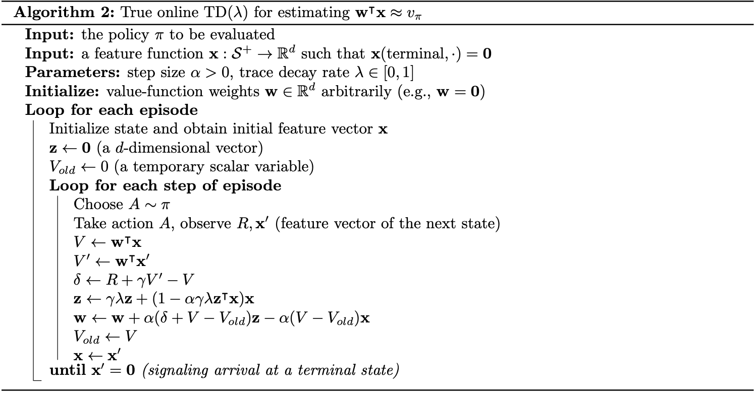
As other methods above, below is an illustration of using true online TD($\lambda$) on the random walk problem.

The eligible trace \eqref{eq:totl.6} is called dutch trace to distinguish it from the trace \eqref{eq:tl.1} of TD($\lambda$), which is called accumulating trace.

There is another kind of trace called replacing trace, defined for the tabular case or for binary feature vectors \begin{equation} z_{i,t}\doteq\begin{cases}1 &\text{if }x_{i,t}=1 \\ \gamma\lambda z_{i,t-1} &\text{if }x_{i,t}=0\end{cases} \end{equation}

Equivalence between forward and backward views

In this section, we will show that there is an interchange between forward and backward view.

Theorem 1
Consider any forward view that updates towards some interim targets $Y_k^t$ with \begin{equation} \mathbf{w}_{k+1}^t=\mathbf{w}_k+\eta_k\left(Y_k^t-\mathbf{x}_k^\text{T}\mathbf{w}_k^t\right)\mathbf{x}_k+\mathbf{u}_k,\hspace{1cm}0\leq k\lt t, \end{equation} where $\mathbf{w}_0^t=\mathbf{w}_0$ for some initial $\mathbf{w}_0$; $\mathbf{u}_k\in\mathbb{R}^d$ is any vector that does not depend on $t$. Assume that the temporal differences $Y_k^{t+1}-Y_k^t$ for different $k$ are related through \begin{equation} Y_k^{t+1}-Y_k^t=c_k(Y_{k+1}^{t+1}-Y_{k+1}^t),\hspace{1cm}\forall k\lt t\label{eq:ebfb.1} \end{equation} where $c_k$ is a scalar that does not depend on $t$. Then the final weights $\mathbf{w}_t^t$ at each time step $t$ are equal to the weight $\mathbf{w}_t$ as defined by $\mathbf{z}_0=\eta_0\mathbf{x}_0$ and the backward view \begin{align} \mathbf{w}_{t+1}&=\mathbf{w}_t+(Y_t^{t+1}-Y_t^t)\mathbf{z}_t+\eta_t(Y_t^t-\mathbf{x}_t^\text{T}\mathbf{w}_t)\mathbf{x}_t+\mathbf{u}_t, \\ \mathbf{z}_t&=c_{t-1}\mathbf{z}_{t-1}+\eta_t\left(1-c_{t-1}\mathbf{x}_t^\text{T}\mathbf{z}_{t-1}\right)\mathbf{x}_t,\hspace{1cm}t\gt 0 \end{align}

Proof
Let $\mathbf{F}_t\doteq\mathbf{I}-\eta_t\mathbf{x}_t\mathbf{x}_t^\text{T}$ be the fading matrix such that $\mathbf{w}_{t+1}=\mathbf{F}_k\mathbf{w}_k^t+\eta_k Y_k^t\mathbf{x}_k$. For each step $t$, we have: \begin{align} \mathbf{w}_{t+1}^{t+1}-\mathbf{w}_t^t&=\mathbf{F}_t\mathbf{w}_t^{t+1}-\mathbf{w}_t^t+\eta_t Y_t^{t+1}\mathbf{x}_t+\mathbf{u}_t \\ &=\mathbf{F}_t(\mathbf{w}_t^{t+1}-\mathbf{w}_t^t)+\eta_t Y_t^{t+1}\mathbf{x}_t+(\mathbf{F}_t-\mathbf{I})\mathbf{w}_t^t+\mathbf{u}_t \\ &=\mathbf{F}_t(\mathbf{w}_t^{t+1}-\mathbf{w}_t^t)+\eta_t Y_t^{t+1}\mathbf{x}_t-\eta_t\mathbf{x}_t\mathbf{x}_t^\text{T}\mathbf{w}_t^t+\mathbf{u}_t \\ &=\mathbf{F}_t(\mathbf{w}_t^{t+1}-\mathbf{w}_t^t)+\eta_t(Y_t^{t+1}-\mathbf{x}_t^\text{T}\mathbf{w}_t^t)\mathbf{x}_t+\mathbf{u}_t\label{eq:ebfb.2} \end{align} We also have that: \begin{align} \mathbf{w}_t^{t+1}-\mathbf{w}_t^t&=\mathbf{F}_{t-1}(\mathbf{w}_{t-1}^{t+1}-\mathbf{w}_{t-1}^t)+\eta_{t-1}(Y_{t-1}^{t+1}-Y_{t-1}^t)\mathbf{x}_{t-1} \\ &=\mathbf{F}_{t-1}\mathbf{F}_{t-2}(\mathbf{w}_{t-1}^{t+1}-\mathbf{w}_{t-1}^t)+\eta_{n-2}(Y_{t-2}^{t+1}-Y_{t-2}^t)\mathbf{F}_{t-1}\mathbf{x}_{t-2}\nonumber \\ &\hspace{1cm}+\eta_{t-1}(Y_{t-1}^{t+1}-Y_{t-1}^t)\mathbf{x}_{t-1} \\ &\hspace{0.3cm}\vdots\nonumber \\ &=\mathbf{F}_{t-1}\dots\mathbf{F}_0(\mathbf{w}_0^{t+1}-\mathbf{w}_0^t)+\sum_{k=0}^{t-1}\eta_k\mathbf{F}_{t-1}\dots\mathbf{F}_{k+1}(Y_k^{t+1}-Y_k^t)\mathbf{x}_k \\ &=\sum_{k=0}^{t-1}\eta_k\mathbf{F}_{t-1}\dots\mathbf{F}_{k+1}(Y_k^{t+1}-Y_k^t)\mathbf{x}_k \\ &=\sum_{k=0}^{t-1}\eta_k\mathbf{F}_{t-1}\dots\mathbf{F}_{k+1}c_k(Y_{k+1}^{t+1}-Y_{k+1}^t)\mathbf{x}_k \\ &\hspace{0.3cm}\vdots\nonumber \\ &=c_{t-1}\underbrace{\sum_{k=0}^{t-1}\eta_k\left(\prod_{j=k}^{t-2}c_j\right)\mathbf{F}_{t-1}\dots\mathbf{F}_{k+1}\mathbf{x}_k}_{\doteq\mathbf{z}_{t-1}}(Y_t^{t+1}-Y_t^t) \\ &=c_{t-1}\mathbf{z}_{t-1}(Y_t^{t+1}-Y_t^t),\label{eq:ebfb.3} \end{align} where in the fifth step, we use the assumption \eqref{eq:ebfb.1}; the vector $\mathbf{z}_t$ defined in the sixth step can be computed recursively in terms of $\mathbf{z}_{t-1}$: \begin{align} \mathbf{z}_t&=\sum_{k=0}^{t}\eta_k\left(\prod_{j=k}^{t-1}c_j\right)\mathbf{F}_1\dots\mathbf{F}_{k+1}\mathbf{x}_k \\ &=\sum_{k=0}^{t-1}\eta_k\left(\prod_{j=k}^{t-1}c_j\right)\mathbf{F}_1\dots\mathbf{F}_{k+1}\mathbf{x}_k+\eta_t\mathbf{x}_t \\ &=c_{t-1}\mathbf{F}_t\sum_{k=0}^{t-1}\eta_k\left(\prod_{j=k}^{t-2}c_j\right)\mathbf{F}_{t-1}\dots\mathbf{F}_{k+1}\mathbf{x}_k+\eta_t\mathbf{x}_t \\ &=c_{t-1}\mathbf{F}_1\mathbf{z}_{t-1}+\eta_t\mathbf{x}_t \\ &=c_{t-1}\mathbf{z}_{t-1}+\eta_t(1-c_{t-1}\mathbf{x}_t^\text{T}\mathbf{z}_{t-1})\mathbf{x}_t \end{align} Plug \eqref{eq:ebfb.3} back into \eqref{eq:ebfb.2} we obtain: \begin{align} \mathbf{w}_{t+1}^{t+1}-\mathbf{w}_t^t&=c_{t-1}\mathbf{F}_t\mathbf{z}_{t-1}(Y_t^{t+1}-Y_t^t)+\eta_t(Y_t^{t+1}-\mathbf{x}_t^\text{T}\mathbf{w}_t)\mathbf{x}_t+\mathbf{u}_t \\ &=(\mathbf{z}_t-\eta_t\mathbf{x}_t)(Y_t^{t+1}-Y_t^t)+\eta_t(Y_t^{t+1}-\mathbf{x}_t^\text{T}\mathbf{w}_t)\mathbf{x}_t+\mathbf{u}_t \\ &=(Y_t^{t+1}-Y_t^t)\mathbf{z}_t+\eta_t(Y_t^t-\mathbf{x}_t^\text{T}\mathbf{w}_t)\mathbf{x}_t+\mathbf{u}_t \end{align} Since $\mathbf{w}_{0,t}\doteq\mathbf{w}_0$, the desired result follows through induction.

Dutch Traces In Monte Carlo

Sarsa($\lambda$)

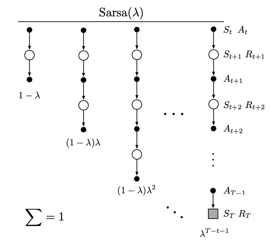
To apply the use off eligible traces on control problems, we begin by defining the $n$-step return, which is the same as what we have defined before: \begin{equation} \hspace{-0.5cm}G_{t:t+n}\doteq\ R_{t+1}+\gamma R_{t+2}+\dots+\gamma^{n-1}R_{t+n}+\gamma^n\hat{q}(S_{t+n},A_{t+n},\mathbf{w}_{t+n-1}),\hspace{1cm}t+n\lt T\label{eq:sl.1} \end{equation} with $G_{t:t+n}\doteq G_t$ if $t+n\geq T$. With this definition of the return, the action-value form of offline $\lambda$-return can be defined as: \begin{equation} \mathbf{w}_{t+1}\doteq\mathbf{w}_t+\alpha\left[G_t^\lambda-\hat{q}(S_t,A_t,\mathbf{w}_t)\right]\nabla_\mathbf{w}\hat{q}(S_t,A_t,\mathbf{w}_t),\hspace{1cm}t=0,\dots,T-1 \end{equation} where $G_t^\lambda\doteq G_{t:\infty}^\lambda$.

The TD method for action values, known as Sarsa($\lambda$), approximates this forward view and has the same update rule as TD($\lambda$): \begin{equation} \mathbf{w}_{t+1}\doteq\mathbf{w}_t+\alpha\delta_t\mathbf{z}_t, \end{equation} except that the TD error, $\delta_t$, is defined in terms of action-value function: \begin{equation} \delta_t\doteq R_{t+1}+\gamma\hat{q}(S_{t+1},A_{t+1},\mathbf{w}_t)-\hat{q}(S_t,A_t,\mathbf{w}_t), \end{equation} and so it is with eligible trace vector: \begin{align} \mathbf{z}_{-1}&\doteq\mathbf{0}, \\ \mathbf{z}&_t\doteq\gamma\lambda\mathbf{z}_{t-1}+\nabla_\mathbf{w}\hat{q}(S_t,A_t,\mathbf{w}_t),\hspace{1cm}0\leq t\lt T \end{align}

Pseudocode of the Sarsa($\lambda$) is given below.

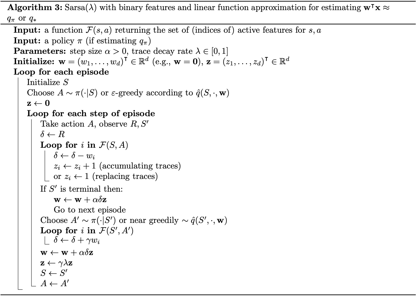
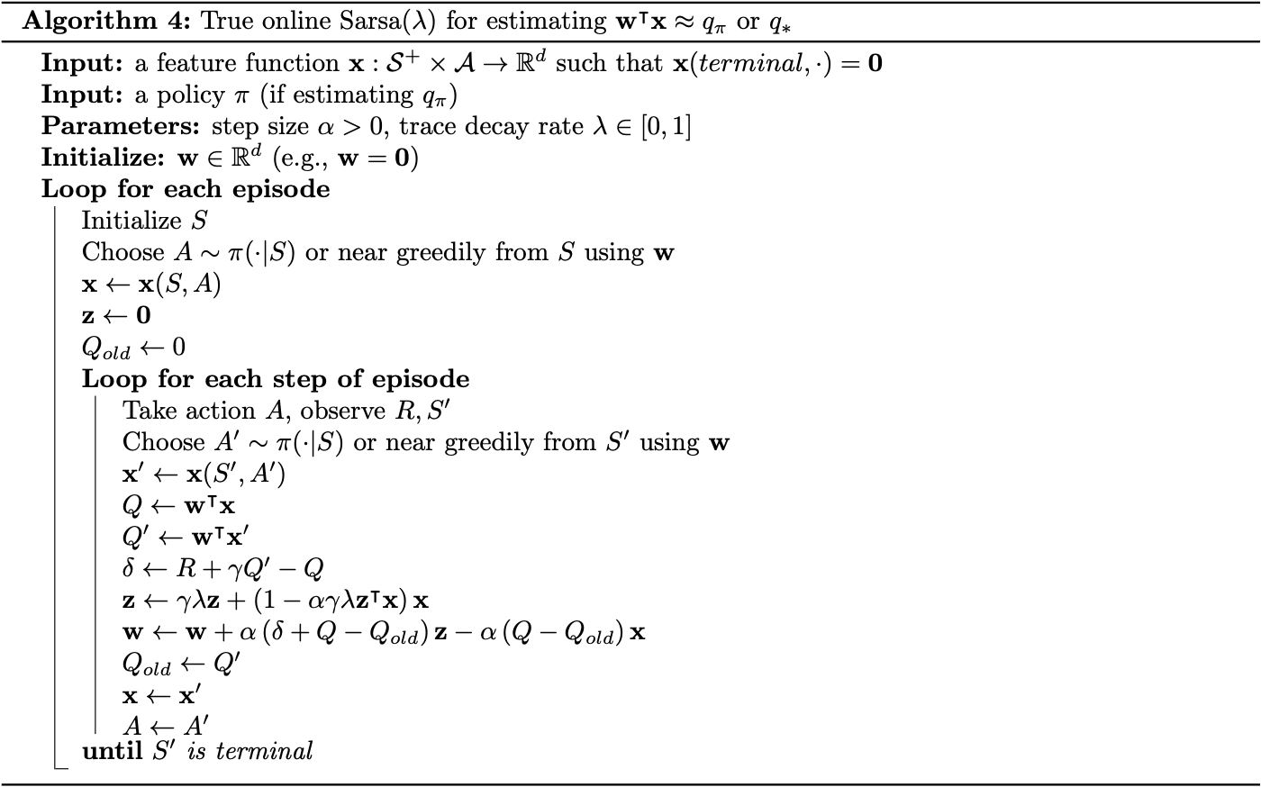
There is also an action-value version of the online $\lambda$-return algorithm, and its efficient implementation as true online TD($\lambda$), called True online Sarsa($\lambda$), which can be achieved by using $n$-step return \eqref{eq:sl.1} instead (which also leads to the change of $\mathbf{x}_t=\mathbf{x}(S_t)$ to $\mathbf{x}_t=\mathbf{x}(S_t,A_t)$).

Pseudocode of the true online Sarsa($\lambda$) is given below.

Variable $\lambda$ and $\gamma$

We can generalize the degree of bootstrapping and discounting beyond constant parameters to functions potentially dependent on the state and action. In other words, each time step $t$, we will have a different $\lambda$ and $\gamma$, denoted as $\lambda_t$ and $\gamma_t$.

In particular, say $\lambda:\mathcal{S}\times\mathcal{A}\to[0,1]$ such that $\lambda_t\doteq\lambda(S_t,A_t)$ and similarly, $\gamma:\mathcal{S}\to[0,1]$ such that $\gamma_t\doteq\gamma(S_t)$.

With this definition of $\gamma$, the return can be rewritten generally as: \begin{align} G_t&\doteq R_{t+1}+\gamma_{t+1}G_{t+1} \\ &=R_{t+1}+\gamma_{t+1}R_{t+2}+\gamma_{t+1}\gamma_{t+2}R_{t+3}+\dots \\ &=\sum_{k=t}^{\infty}\left(\prod_{i=t+1}^{k}\gamma_i\right)R_{k+1}, \end{align} where we require that $\prod_{k=t}^{\infty}\gamma_k=0$ with probability $1$ for all $t$ to assure the sums are finite.

The generalization of $\lambda$ also lets us rewrite the state-based $\lambda$-return as: \begin{equation} G_t^{\lambda s}\doteq R_{t+1}+\gamma_{t+1}\Big((1-\lambda_{t+1})\hat{v}(S_{t+1},\mathbf{w}_t)+\lambda_{t+1}G_{t+1}^{\lambda s}\Big),\label{eq:lg.1} \end{equation} where $G_t^{\lambda s}$ denotes that this $\lambda$ -return is bootstrapped from state values, and hence the $G_t^{\lambda a}$ denotes the $\lambda$-return that bootstraps from action values. The Sarsa form of action-based $\lambda$-return is defined as: \begin{equation} G_t^{\lambda a}\doteq R_{t+1}+\gamma_{t+1}\Big((1-\lambda_{t+1})\hat{q}(S_{t+1},A_{t+1},\mathbf{w}_t)+\lambda_{t+1}G_{t+1}^{\lambda a}\Big), \end{equation} and the Expected Sarsa form of its can be defined as: \begin{equation} G_t^{\lambda a}\doteq R_{t+1}+\gamma_{t+1}\Big((1-\lambda_{t+1})\overline{V}_t(S_{t+1})+\lambda_{t+1}G_{t+1}^{\lambda a}\Big),\label{eq:lg.2} \end{equation} where the expected approximate value is generalized to function approximation as: \begin{equation} \overline{V}_t\doteq\sum_a\pi(a|s)\hat{q}(s,a,\mathbf{w}_t)\label{eq:lg.3} \end{equation}

Off-policy Traces with Control Variates

We can also apply the use of importance sampling with eligible traces.

We begin with the new definition of $\lambda$-return, which is achieved by generalizing the $\lambda$-return \eqref{eq:lg.1} with the idea of control variates on $n$-step off-policy return: \begin{equation} \hspace{-0.5cm}G_t^{\lambda s}\doteq\rho_t\Big(R_{t+1}+\gamma_{t+1}\big((1-\lambda_{t+1})\hat{v}(S_{t+1},\mathbf{w}_t)+\lambda_{t+1}G_{t+1}^{\lambda s}\big)\Big)+(1-\rho_t)\hat{v}(S_t,\mathbf{w}_t), \end{equation} where the single-step importance sampling ratio $\rho_t$ is defined as usual: \begin{equation} \rho_t\doteq\frac{\pi(A_t|S_t)}{b(A_t|S_t)} \end{equation} Much like the other returns, the truncated version of this return can be approximated simply in terms of sums of state-based TD errors: \begin{equation} G_t^{\lambda s}\approx\hat{v}(S_t,\mathbf{w}_t)+\rho_t\sum_{k=t}^{\infty}\delta_k^s\prod_{i=t+1}^{k}\gamma_i\lambda_i\rho_i, \end{equation} where the state-based TD error, $\delta_t^s$, is defined as: \begin{equation} \delta_t^s\doteq R_{t+1}+\gamma_{t+1}\hat{v}(S_{t+1},\mathbf{w}_t)-\hat{v}(S_t,\mathbf{w}_t),\label{eq:optcv.1} \end{equation} with the approximation becoming exact if the approximate value function does not change. Given this approximation, we have that: \begin{align} \mathbf{w}_{t+1}&=\mathbf{w}_t+\alpha\left(G_t^{\lambda s}-\hat{v}(S_t,\mathbf{w}_t)\right)\nabla_\mathbf{w}\hat{v}(S_t,\mathbf{w}_t) \\ &\approx\mathbf{w}_t+\alpha\rho_t\left(\sum_{k=t}^{\infty}\delta_k^s\prod_{i=t+1}^{k}\gamma_i\lambda_i\rho_i\right)\nabla_\mathbf{w}\hat{v}(S_t,\mathbf{w}_t) \end{align} This is one time step of a forward view. And in fact, the forward-view update, summed over time, is approximately equal to a backward-view update, summed over time. Since the sum of the forward-view update over time is: \begin{align} \sum_{t=1}^{\infty}(\mathbf{w}_{t+1}-\mathbf{w}_t)&\approx\sum_{t=1}^{\infty}\sum_{k=t}^{\infty}\alpha\rho_t\delta_k^s\nabla_\mathbf{w}\hat{v}(S_t,\mathbf{w}_t)\prod_{i=t+1}^{k}\gamma_i\lambda_i\rho_i \\ &=\sum_{k=1}^{\infty}\sum_{t=1}^{k}\alpha\rho_t\nabla_\mathbf{w}\hat{v}(S_t,\mathbf{w}_t)\delta_k^s\prod_{i=t+1}^{k}\gamma_i\lambda_i\rho_i \\ &=\sum_{k=1}^{\infty}\alpha\delta_k^s\sum_{t=1}^{k}\nabla_\mathbf{w}\hat{v}(S_t,\mathbf{w}_t)\prod_{i=t+1}^{k}\gamma_i\lambda_i\rho_i,\label{eq:optcv.2} \end{align} where in the second step, we use the summation rule: $\sum_{t=x}^{y}\sum_{k=t}^{y}=\sum_{k=x}^{y}\sum_{t=x}^{k}$.

Let $\mathbf{z}_k$ is defined as: \begin{align} \mathbf{z}_k &=\sum_{t=1}^{k}\rho_t\nabla_\mathbf{w}\hat{v}\left(S_t, \mathbf{w}_t\right)\prod_{i=t+1}^{k} \gamma_i\lambda_i\rho_i \\ &=\sum_{t=1}^{k-1}\rho_t\nabla_\mathbf{w}\hat{v}\left(S_t,\mathbf{w}_t\right)\prod_{i=t+1}^{k}\gamma_i\lambda_i\rho_i+\rho_k\nabla_\mathbf{w}\hat{v}\left(S_k,\mathbf{w}_k\right) \\ &=\gamma_k\lambda_k\rho_k\underbrace{\sum_{t=1}^{k-1}\rho_t\nabla_\mathbf{w}\hat{v}\left(S_t,\mathbf{w}_t\right)\prod_{i=t+1}^{k-1}\gamma_i\lambda_i\rho_i}_{\mathbf{z}_{k-1}}+\rho_k\nabla_\mathbf{w}\hat{v}\left(S_k,\mathbf{w}_k\right) \\ &=\rho_k\big(\gamma_k\lambda_k\mathbf{z}_{k-1}+\nabla_\mathbf{w}\hat{v}\left(S_k,\mathbf{w}_k\right)\big) \end{align} Then we can rewrite \eqref{eq:optcv.2} as: \begin{equation} \sum_{t=1}^{\infty}\left(\mathbf{w}_{t+1}-\mathbf{w}_t\right)\approx\sum_{k=1}^{\infty}\alpha\delta_k^s\mathbf{z}_k, \end{equation} which is sum of the backward-view update over time, with the eligible trace vector is defined as: \begin{equation} \mathbf{z}_t\doteq\rho_t\big(\gamma_t\lambda_t\mathbf{z}_{t-1}+\nabla_\mathbf{w}\hat{v}(S_t,\mathbf{w}_t)\big)\label{eq:optcv.3} \end{equation} Using this eligible trace with the parameter update rule \eqref{eq:tl.2} of TD($\lambda$), we obtain a general TD($\lambda$) algorithm that can be applied to either on-policy or off-policy data.

• In the on-policy case, the algorithm is exactly TD($\lambda$) because $\rho_t=1$ for all $t$ and \eqref{eq:optcv.3} becomes the accumulating trace \eqref{eq:tl.1} with extending to variable $\lambda$ and $\gamma$.
• In the off-policy case, the algorithm often works well but, as a semi-gradient method, is not guaranteed to be stable.

For action-value function, we generalize the definition of the $\lambda$-return \eqref{eq:lg.2} of Expected Sarsa with the idea of control variate: \begin{align} G_t^{\lambda a}&\doteq R_{t+1}+\gamma_{t+1}\Big((1-\lambda_{t+1})\bar{V}_t(S_{t+1})+\lambda_{t+1}\big[\rho_{t+1}G_{t+1}^{\lambda a}+\bar{V}_t(S_{t+1})\nonumber \\ &\hspace{2cm}-\rho_{t+1}\hat{q}(S_{t+1},A_{t+1},\mathbf{w}_t)\big]\Big) \\ &=R_{t+1}+\gamma_{t+1}\Big(\bar{V}_t(S_{t+1})+\lambda_{t+1}\rho_{t+1}\left[G_{t+1}^{\lambda a}-\hat{q}(S_{t+1},A_{t+1},\mathbf{w}_t)\right]\Big), \end{align} where the expected approximate value $\bar{V}_t(S_{t+1})$ is as given by \eqref{eq:lg.3}.

Similar to the others, this $\lambda$-return can also be written approximately as the sum of TD errors \begin{equation} G_t^{\lambda a}\approx\hat{q}(S_t,A_t,\mathbf{w}_t)+\sum_{k=t}^{\infty}\delta_k^a\prod_{i=t+1}^{k}\gamma_i\lambda_i\rho_i, \end{equation} with the action-based TD error is defined in terms of the expected approximate value: \begin{equation} \delta_t^a=R_{t+1}+\gamma_{t+1}\bar{V}_t(S_{t+1})-\hat{q}(S_t,A_t,\mathbf{w}_t)\label{eq:optcv.4} \end{equation} Analogy to the state value function case, this approximation also becomes exact if the approximate value function does not change.

Similar to the state case \eqref{eq:optcv.3}, we can also define the eligible trace for action values: \begin{equation} \mathbf{z}_t\doteq\gamma_t\lambda_t\rho_t\mathbf{z}_{t-1}+\nabla_\mathbf{w}\hat{q}(S_t,A_t,\mathbf{w}_t) \end{equation} Using this eligible trace with the parameter update rule \eqref{eq:tl.2} of TD($\lambda$) and the expectation-based TD error \eqref{eq:optcv.4}, we end up with an Expected Sarsa($\lambda$) algorithm that can applied to either on-policy or off-policy data.

• In the on-policy case with constant $\lambda$ and $\gamma$, this becomes the Sarsa($\lambda$) algorithm.

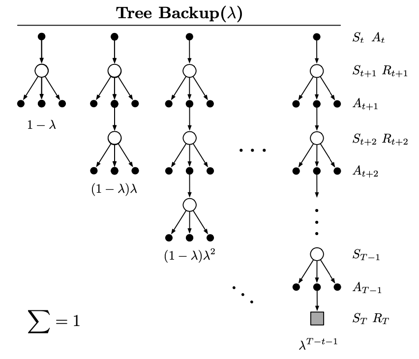
Tree-Backup($\lambda$)

Recall that in the note of TD-Learning, we have mentioned that there is an off-policy method without importance sampling called tree-backup. Can we extend the idea of tree-backup to an eligible trace version? Yes, we can.

As usual, we begin with establishing the $\lambda$-return by generalizing the $\lambda$-return of Expected Sarsa \eqref{eq:lg.2} with the $n$-step Tree-backup return: \begin{align} G_t^{\lambda a}&\doteq R_{t+1}+\gamma_{t+1}\Bigg((1-\lambda_{t+1})\bar{V}_t(S_{t+1})+\lambda_{t+1}\Big[\sum_{a\neq A_{t+1}}\pi(a|S_{t+1})\hat{q}(S_{t+1},a,\mathbf{w}_t)\nonumber \\ &\hspace{2cm}+\pi(A_{t+1}|S_{t+1})G_{t+1}^{\lambda a}\Big]\Bigg) \\ &=R_{t+1}+\gamma_{t+1}\Big(\bar{V}_t(S_{t+1})+\lambda_{t+1}\pi(A_{t+1}|S_{t+1})\left(G_{t+1}^{\lambda a}-\hat{q}(S_{t+1},A_{t+1},\mathbf{w}_t)\right)\Big) \end{align} This return, as usual, can also be written approximately (ignoring changes in the approximate value function) as sum of TD errors: \begin{equation} G_t^{\lambda a}\approx\hat{q}(S_t,A_t,\mathbf{w}_t)+\sum_{k=t}^{\infty}\delta_k^a\prod_{i=t+1}^{k}\gamma_i\lambda_i\pi(A_i|S_i), \end{equation} with the TD error is defined as given by \eqref{eq:optcv.4}.

Similar to how we derive the eligible trace \eqref{eq:optcv.3}, we can define a new eligible trace in terms of target-policy probabilities of the selected actions: \begin{equation} \mathbf{z}_t\doteq\gamma_t\lambda_t\pi(A_t|S_t)\mathbf{z}_{t-1}+\nabla_\mathbf{w}\hat{q}(S_t,A_t,\mathbf{w}_t) \end{equation} Using this eligible trace vector with the parameter update rule \eqref{eq:tl.2} of TD($\lambda$), we end up with the Tree-Backup($\lambda$) or TB($\lambda$).

Other Off-policy Methods with Traces

GTD($\lambda$)

GTD($\lambda$) is the extended version of TDC, a state-value Gradient-TD method, with eligible traces.

In this algorithm, we will define a new off-policy, $\lambda$-return, not like usual but as a function: \begin{equation} G_t^{\lambda}(v)\doteq R_{t+1}+\gamma_{t+1}\Big[(1-\lambda_{t+1})v(S_{t+1})+\lambda_{t+1}G_{t+1}^{\lambda}(v)\Big]\label{eq:gl.1} \end{equation} where $v(s)$ denotes the value at state $s$, and $\lambda\in[0,1]$ is the trace-decay parameter.

Let $T_\pi^\lambda$ denote the $\lambda$-weighted Bellman operator for policy $\pi$ such that: \begin{align} v_\pi(s)&=\mathbb{E}\Big[G_t^\lambda(v_\pi)\big|S_t=s,\pi\Big] \\ &\doteq (T_\pi^\lambda v_\pi)(s) \end{align}

Consider using linear function approximation, or in particular, we are trying to approximate $v(s)$ by $v_\mathbf{w}(s)=\mathbf{w}^\text{T}\mathbf{x}(s)$. Our objective is to find the fixed-point which satisfies: \begin{equation} v_\mathbf{w}=\Pi T_\pi^\lambda v_\mathbf{w},\label{eq:gl.2} \end{equation} where $\Pi v$ is a projection of $v$ into the space of representable functions $\{v_\mathbf{w}|\mathbf{w}\in\mathbb{R}^d\}$. Let $\mu$ be the steady-state distribution of states under the behavior policy $b$. Then, the projection can be defined as: \begin{equation} \Pi v\doteq v_{\mathbf{w}}, \end{equation} where \begin{equation} \mathbf{w}=\underset{\mathbf{w}\in\mathbb{R}^d}{\text{argmin}}\left\Vert v-v_\mathbf{w}\right\Vert_\mu^2, \end{equation} In a linear case, in which $v_\mathbf{w}=\mathbf{X}\mathbf{w}$, the projection operator is linear and independent of $\mathbf{w}$: \begin{equation} \Pi=\mathbf{X}(\mathbf{X}^\text{T}\mathbf{D}\mathbf{X})^{-1}\mathbf{X}^\text{T}\mathbf{D}, \end{equation} where $\mathbf{D}$ denotes $\vert\mathcal{S}\vert\times\vert\mathcal{S}\vert$ diagonal matrix whose diagonal elements are $\mu(s)$, and $\mathbf{X}$ denotes the $\vert\mathcal{S}\vert\times d$ matrix whose rows are the feature vectors $\mathbf{x}(s)^\text{T}$, one for each state $s$.

With linear function approximation, we can rewrite the $\lambda$-return \eqref{eq:gl.1} as: \begin{equation} G_t^{\lambda}(\mathbf{w})\doteq R_{t+1}+\gamma_{t+1}\Big[(1-\lambda_{t+1})\mathbf{w}^\text{T}\mathbf{x}_{t+1}+\lambda_{t+1}G_{t+1}^{\lambda}(\mathbf{w})\Big]\label{eq:gl.3} \end{equation} Let \begin{equation} \delta_t^\lambda(\mathbf{w})\doteq G_t^\lambda(\mathbf{w})-\mathbf{w}^\text{T}\mathbf{x}_t, \end{equation} and \begin{equation} \mathcal{P}_\mu^\pi\delta_t^\lambda(\mathbf{w})\mathbf{x}_t\doteq\sum_s\mu(s)\mathbb{E}\Big[\delta_t^\lambda(\mathbf{w})\big|S_t=s,\pi\Big]\mathbf{x}(s), \end{equation} where $\mathcal{P}_\mu^\pi$ is an operator.

The fixed-point in \eqref{eq:gl.2} can be found by minimizing the Mean Square Projected Bellman Error (MSPBE): \begin{align} \overline{\text{PBE}}(\mathbf{w})&=\Big\Vert v_\mathbf{w}-\Pi T_\pi^\lambda v_\mathbf{w}\Big\Vert_\mu^2 \\ &=\Big\Vert\Pi(v_\mathbf{w}-T_\pi^\lambda v_\mathbf{w})\Big\Vert_\mu^2 \\ &=\Big(\Pi\left(v_\mathbf{w}-T_\pi^\lambda v_\mathbf{w}\right)\Big)^\text{T}\mathbf{D}\Big(\Pi\left(v_\mathbf{w}-T_\pi^\lambda v_\mathbf{w}\right)\Big) \\ &=\left(v_\mathbf{w}-T_\pi^\lambda v_\mathbf{w}\right)^\text{T}\Pi^\text{T}\mathbf{D}\Pi\left(v_\mathbf{w}-T_\pi^\lambda v_\mathbf{w}\right) \\ &=\left(v_\mathbf{w}-T_\pi^\lambda v_\mathbf{w}\right)^\text{T}\mathbf{D}^\text{T}\mathbf{X}\left(\mathbf{X}^\text{T}\mathbf{D}\mathbf{X}\right)^{-1}\mathbf{D}\left(v_\mathbf{w}-T_\pi^\lambda v_\mathbf{w}\right) \\ &=\Big(\mathbf{X}^\text{T}\mathbf{D}\left(T_\pi^\lambda v_\mathbf{w}-\mathbf{w}\right)\Big)^\text{T}\left(\mathbf{X}^\text{T}\mathbf{D}\mathbf{X}\right)^{-1}\mathbf{X}^\text{T}\mathbf{D}\left(T_\pi^\lambda v_\mathbf{w}-v_\mathbf{w}\right)\label{eq:gl.4} \end{align}

From the definition of $T_\pi^\lambda$ and $\delta_t^\lambda$, we have: \begin{align} (T_\pi^\lambda v_\mathbf{w}-v_\mathbf{v})(s)&=\mathbb{E}\Big[G_t^\lambda(\mathbf{w})-\mathbf{w}^\text{T}\mathbf{x}_t\big|S_t=s,\pi\Big] \\ &=\mathbb{E}\Big[\delta_t^\lambda(\mathbf{w})\big|S_t=s,\pi\Big]\label{eq:gl.5} \end{align} Therefore, \begin{align} \mathbf{X}^\text{T}\mathbf{D}\left(T_\pi^\lambda v_\mathbf{w}-v_\mathbf{w}\right)&=\sum_s\mu(s)\Big[\left(T_\pi^\lambda v_\mathbf{w}-v_\mathbf{w}\right)(s)\Big]\mathbf{x}(s) \\ &=\sum_s\mu(s)\mathbb{E}\Big[\delta_t^\lambda(\mathbf{w})|S_t=s,\pi\Big]\mathbf{x}(s) \\ &=\mathcal{P}_\mu^\pi\delta_t^\lambda(\mathbf{w})\mathbf{x}_t\label{eq:gl.6} \end{align} Moreover, we also have: \begin{equation} \mathbf{X}^\text{T}\mathbf{D}\mathbf{X}=\sum_s\mu(s)\mathbf{x}(s)\mathbf{x}(s)^\text{T}=\mathbb{E}\Big[\mathbf{x}_t\mathbf{x}_t^\text{T}\Big]\label{eq:gl.7} \end{equation} Substitute \eqref{eq:gl.5}, \eqref{eq:gl.6} and \eqref{eq:gl.7} back to the \eqref{eq:gl.4}, we have: \begin{equation} \overline{\text{PBE}}(\mathbf{w})=\Big(\mathcal{P}_\mu^\pi\delta_t^\lambda(\mathbf{w})\mathbf{x}_t\Big)^\text{T}\mathbb{E}\Big[\mathbf{x}_t\mathbf{x}_t^\text{T}\Big]^{-1}\Big(\mathcal{P}_\mu^\pi\delta_t^\lambda(\mathbf{w})\mathbf{x}_t\Big)\label{eq:gl.8} \end{equation} In the objective function \eqref{eq:gl.8}, the expectation terms are w.r.t the policy $\pi$, while the data is generated due to the behavior policy $b$. To solve this off-policy problem, as usual, we use importance sampling.

We then instead use an importance-sampling version of $\lambda$-return \eqref{eq:gl.3}: \begin{equation} G_t^{\lambda\rho}(\mathbf{w})=\rho_t\left(R_{t+1}+\gamma_{t+1}\left[(1-\lambda_{t+1})\mathbf{w}^\text{T}\mathbf{x}_{t+1}+\lambda_{t+1}G_{t+1}^{\lambda\rho}(\mathbf{w})\right]\right), \end{equation} where the single-step importance sampling ratio $\rho_t$ is defined as usual: \begin{equation} \rho_t\doteq\frac{\pi(A_t|S_t)}{b(A_t|S_t)} \end{equation} This also leads to an another version of $\delta_t^\lambda$, defined as: \begin{equation} \delta_t^{\lambda\rho}(\mathbf{w})\doteq G_t^{\lambda\rho}(\mathbf{w})-\mathbf{w}^\text{T}\mathbf{x}_t \end{equation} With this definition of the $\lambda$-return, we have: \begin{align} &\hspace{-1cm}\mathbb{E}\Big[G_t^{\lambda\rho}(\mathbf{w})\big|S_t=s\Big]\nonumber \\ &\hspace{-1cm}=\mathbb{E}\Big[\rho_t\big(R_{t+1}+\gamma_{t+1}(1-\lambda_{t+1})\mathbf{w}^\text{T}\mathbf{x}_{t+1}\big)+\rho_t\gamma_{t+1}\lambda_{t+1}G_{t+1}^{\lambda\rho}(\mathbf{w})\big|S_t=s\Big] \\ &\hspace{-1cm}=\mathbb{E}\Big[\rho_t\big(R_{t+1}+\gamma_{t+1}(1-\lambda_{t+1})\mathbf{w}^\text{T}\mathbf{x}_{t+1}\big)\big|S_t=s\Big]+\rho_t\gamma_{t+1}\lambda_{t+1}\mathbb{E}\Big[G_{t+1}^{\lambda\rho}(\mathbf{w})\big|S_t=s\Big] \\ &\hspace{-1cm}=\mathbb{E}\Big[R_{t+1}+\gamma_{t+1}(1-\lambda_{t+1})\mathbf{w}^\text{T}\mathbf{x}_{t+1}\big|S_t=s,\pi\Big]\nonumber \\ &\hspace{1cm}+\sum_{a,s’}p(s’|s,a)b(a|s)\frac{\pi(a|s)}{b(a|s)}\gamma_{t+1}\lambda_{t+1}\mathbb{E}\Big[G_{t+1}^{\lambda\rho}(\mathbf{w})\big|S_{t+1}=s’\Big] \\ &\hspace{-1cm}=\mathbb{E}\Big[R_{t+1}+\gamma_{t+1}(1-\lambda_{t+1})\mathbf{w}^\text{T}\mathbf{x}_{t+1}\big|S_t=s,\pi\Big]\nonumber \\ &\hspace{1cm}+\sum_{a,s’}p(s’|s,a)\pi(a|s)\gamma_{t+1}\lambda_{t+1}\mathbb{E}\Big[G_{t+1}^{\lambda\rho}(\mathbf{w})\big|S_{t+1}=s’\Big] \\ &\hspace{-1cm}=\mathbb{E}\Big[R_{t+1}+\gamma_{t+1}(1-\lambda_{t+1})\mathbf{w}^\text{T}\mathbf{x}_{t+1}+\gamma_{t+1}\lambda_{t+1}\mathbb{E}\Big[G_{t+1}^{\lambda\rho}(\mathbf{w})\big|S_{t+1}=s’\Big]\big|S_t=s,\pi\Big], \end{align} which, as it continues to roll out, gives us: \begin{equation} \mathbb{E}\Big[G_t^{\lambda\rho}(\mathbf{w})\big|S_t=s\Big]=\mathbb{E}\Big[G_t^{\lambda}(\mathbf{w})\big|S_t=s,\pi\Big] \end{equation} And eventually, we get: \begin{equation} \mathbb{E}\Big[\delta_t^{\lambda\rho}(\mathbf{w})\mathbf{x}_t\Big]=\mathcal{P}_\mu^\pi\delta_t^\lambda(\mathbf{w})\mathbf{x}_t \end{equation} because the state distribution is based on behavior state-distribution $\mu$.

With this result, our objective function \eqref{eq:gl.8} can be written as: \begin{align} \overline{\text{PBE}}(\mathbf{w})&=\Big(\mathcal{P}_\mu^\pi\delta_t^\lambda(\mathbf{w})\mathbf{x}_t\Big)^\text{T}\mathbb{E}\Big[\mathbf{x}_t\mathbf{x}_t^\text{T}\Big]^{-1}\Big(\mathcal{P}_\mu^\pi\delta_t^\lambda(\mathbf{w})\mathbf{x}_t\Big) \\ &=\mathbb{E}\Big[\delta_t^{\lambda\rho}(\mathbf{w})\mathbf{x}_t\Big]^\text{T}\mathbb{E}\Big[\mathbf{x}_t\mathbf{x}_t^\text{T}\Big]^{-1}\mathbb{E}\Big[\delta_t^{\lambda\rho}(\mathbf{w})\mathbf{x}_t\Big]\label{eq:gl.9} \end{align} From the definition of $\delta_t^{\lambda\rho}$, we have: \begin{align} \delta_t^{\lambda\rho}(\mathbf{w})&=G_t^{\lambda\rho}(\mathbf{w})-\mathbf{w}^\text{T}\mathbf{x}_t \\ &=\rho_t\Big(R_{t+1}+\gamma_{t+1}\big[(1-\lambda_{t+1})\mathbf{w}^\text{T}\mathbf{x}_{t+1}+\lambda_{t+1}G_{t+1}^{\lambda\rho}(\mathbf{w})\big]\Big)-\mathbf{w}^\text{T}\mathbf{x}_t \\ &=\rho_t\Big(R_{t+1}+\gamma_{t+1}\mathbf{w}^\text{T}\mathbf{x}_{t+1}-\mathbf{w}^\text{T}\mathbf{x}_t+\mathbf{w}^\text{T}\mathbf{x}_t\Big)\nonumber \\ &\hspace{2cm}-\rho_t\gamma_{t+1}\lambda_{t+1}\mathbf{w}^\text{T}\mathbf{x}_{t+1}+\rho_t\gamma_{t+1}\lambda_{t+1}G_{t+1}^{\lambda\rho}(\mathbf{w})-\mathbf{w}^\text{T}\mathbf{x}_t \\ &=\rho_t\Big(R_{t+1}+\gamma_{t+1}\mathbf{w}^\text{T}\mathbf{x}_{t+1}-\mathbf{w}^\text{T}\mathbf{x}_t\Big)+\rho_t\mathbf{w}^\text{T}\mathbf{x}_t-\mathbf{w}^\text{T}\mathbf{x}_t\nonumber \\ &\hspace{2cm}+\rho_t\gamma_{t+1}\lambda_{t+1}\Big(G_{t+1}^{\lambda\rho}(\mathbf{w})-\mathbf{w}^\text{T}\mathbf{x}_{t+1}\Big) \\ &=\rho_t\delta_t(\mathbf{w})+(\rho_t-1)\mathbf{w}^\text{T}\mathbf{x}_t+\rho_t\gamma_{t+1}\lambda_{t+1}\delta_{t+1}^{\lambda\rho}(\mathbf{w}), \end{align} where the TD error, $\delta_t(\mathbf{w})$, is defined as usual: \begin{equation} \delta_t(\mathbf{w})\doteq R_{t+1}+\gamma_{t+1}\mathbf{w}^\text{T}\mathbf{x}_{t+1}-\mathbf{w}^\text{T}\mathbf{x}_t \end{equation} Also, we have that: \begin{align} \mathbb{E}\Big[(1-\rho_t)\mathbf{w}^\text{T}\mathbf{x}_t\mathbf{x}_t\Big]&=\sum_{s,a}\mu(s)b(a|s)\left(1-\frac{\pi(a|s)}{b(a|s)}\right)\mathbf{w}^\text{T}\mathbf{x}(s)\mathbf{x}(s) \\ &=\sum_s\mu(s)\left(\sum_a b(a|s)-\sum_a\pi(a|s)\right)\mathbf{w}^\text{T}\mathbf{x}(s)\mathbf{x}(s) \\ &=\sum_s\mu(s)(1-1)\mathbf{w}^\text{T}\mathbf{x}(s)\mathbf{x}(s) \\ &=0 \end{align} Given these results, we have: \begin{align} \hspace{-1cm}\mathbb{E}\Big[\delta_t^{\lambda\rho}(\mathbf{w})\mathbf{x}_t\Big]&=\mathbb{E}\Big[\rho_t\delta_t(\mathbf{w})\mathbf{x}_t+(\rho_t-1)\mathbf{w}^\text{T}\mathbf{x}_t\mathbf{x}_t+\rho_t\gamma_{t+1}\lambda_{t+1}\delta_{t+1}^{\lambda\rho}(\mathbf{w})\mathbf{x}_t\Big] \\ &=\mathbb{E}\Big[\rho_t\delta_t(\mathbf{w})\mathbf{x}_t\Big]+0+\mathbb{E}_{\pi b}\Big[\rho_t\gamma_{t+1}\lambda_{t+1}\delta_{t+1}^{\lambda\rho}(\mathbf{w})\mathbf{x}_t\Big] \\ &=\mathbb{E}\Big[\rho_t\delta_t(\mathbf{w})\mathbf{x}_t+\rho_{t-1}\gamma_t\lambda_t\delta_t^{\lambda\rho}(\mathbf{w})\mathbf{x}_{t-1}\Big] \\ &=\mathbb{E}\Big[\rho_t\delta_t(\mathbf{w})\mathbf{x}_t+\rho_{t-1}\gamma_t\lambda_t\big(\rho_t\delta_t(\mathbf{w})+(\rho_t-1)\mathbf{w}^\text{T}\mathbf{x}_t\nonumber \\ &\hspace{2cm}+\rho_t\gamma_{t+1}\lambda_{t+1}\delta_{t+1}^{\lambda\rho}(\mathbf{w})\big)\mathbf{x}_{t-1}\Big] \\ &=\mathbb{E}\Big[\rho_t\delta_t(\mathbf{w})\mathbf{x}_t+\rho_{t-1}\gamma_t\lambda_t\big(\rho_t\delta_t(\mathbf{w})+\rho_t\gamma_{t+1}\lambda_{t+1}\delta_{t+1}^{\lambda\rho}(\mathbf{w})\big)\mathbf{x}_{t-1}\Big] \\ &=\mathbb{E}\Big[\rho_t\delta_t(\mathbf{w})\big(\mathbf{x}_t+\rho_{t-1}\gamma_t\lambda_t\mathbf{x}_{t-1}\big)+\rho_{t-1}\gamma_t\lambda_t\rho_t\gamma_{t+1}\lambda_{t+1}\delta_{t+1}^{\lambda\rho}(\mathbf{w})\mathbf{x}_{t-1}\Big] \\ &=\mathbb{E}\Big[\rho_t\delta_t(\mathbf{w})\big(\mathbf{x}_t+\rho_{t-1}\gamma_t\lambda_t\mathbf{x}_{t-1}\big)+\rho_{t-2}\gamma_{t-1}\lambda_{t-1}\rho_{t-1}\gamma_t\lambda_t\delta_t^{\lambda\rho}(\mathbf{w})\mathbf{x}_{t-2}\Big] \\ &\hspace{0.3cm}\vdots\nonumber \\ &=\mathbb{E}\Big[\delta_t(\mathbf{w})\rho_t\big(\mathbf{x}_t+\rho_{t-1}\gamma_t\lambda_t\mathbf{x}_{t-1}+\rho_{t-2}\gamma_{t-1}\lambda_{t-1}\rho_{t-1}\gamma_t\lambda_t\mathbf{x}_{t-2}+\dots\big)\Big] \\ &=\mathbb{E}\Big[\delta_t(\mathbf{w})\mathbf{z}_t\Big], \end{align} where \begin{equation} \mathbf{z}_t=\rho_t(\mathbf{x}_t+\gamma_t\lambda_t\mathbf{z}_{t-1}) \end{equation} Plugging this result back to \eqref{eq:gl.9} lets our objective function become: \begin{equation} \overline{\text{PBE}}(\mathbf{w})=\mathbb{E}\Big[\delta_t(\mathbf{w})\mathbf{z}_t\Big]^\text{T}\mathbb{E}\Big[\mathbf{x}_t\mathbf{x}_t^\text{T}\Big]^{-1}\mathbb{E}\Big[\delta_t(\mathbf{w})\mathbf{z}_t\Big]\label{eq:gl.10} \end{equation} Similar to TDC, we also use gradient descent in order to find the minimum value of $\overline{\text{PBE}}(\mathbf{w})$. The gradient of our objective function w.r.t the weight vector $\mathbf{w}$ is: \begin{align} \hspace{-1.2cm}\frac{1}{2}\nabla_\mathbf{w}\overline{\text{PBE}}(\mathbf{w})&=-\frac{1}{2}\nabla_\mathbf{w}\Bigg(\mathbb{E}\Big[\delta_t(\mathbf{w})\mathbf{z}_t\Big]^\text{T}\mathbb{E}\Big[\mathbf{x}_t\mathbf{x}_t^\text{T}\Big]^{-1}\mathbb{E}\Big[\delta_t(\mathbf{w})\mathbf{z}_t\Big]\Bigg) \\ &=\nabla_\mathbf{w}\mathbb{E}\Big[\delta_t(\mathbf{w})\mathbf{z}_t^\text{T}\Big]\mathbb{E}\Big[\mathbf{x}_t\mathbf{x}_t^\text{T}\Big]^{-1}\mathbb{E}\Big[\delta_t(\mathbf{w})\mathbf{z}_t\Big] \\ &=-\mathbb{E}\Big[\big(\gamma_{t+1}\mathbf{x}_{t+1}-\mathbf{x}_t\big)\mathbf{z}_t^\text{T}\Big]\mathbb{E}\Big[\mathbf{x}_t\mathbf{x}_t^\text{T}\Big]^{-1}\mathbb{E}\Big[\delta_t(\mathbf{w})\mathbf{z}_t\Big] \\ &=-\mathbb{E}\Big[\gamma_{t+1}\mathbf{x}_{t+1}\mathbf{z}_t^\text{T}-\mathbf{x}_t\mathbf{z}_t^\text{T}\Big]\mathbb{E}\Big[\mathbf{x}_t\mathbf{x}_t^\text{T}\Big]^{-1}\mathbb{E}\Big[\delta_t(\mathbf{w})\mathbf{z}_t\Big] \\ &=-\mathbb{E}\Big[\gamma_{t+1}\mathbf{x}_{t+1}\mathbf{z}_t^\text{T}-\mathbf{x}_t\rho_t\big(\mathbf{x}_t+\gamma_t\lambda_t\mathbf{z}_{t-1}\big)^\text{T}\Big]\mathbb{E}\Big[\mathbf{x}_t\mathbf{x}_t^\text{T}\Big]^{-1}\mathbb{E}\Big[\delta_t(\mathbf{w})\mathbf{z}_t\Big] \\ &=-\mathbb{E}\Big[\gamma_{t+1}\mathbf{x}_{t+1}\mathbf{z}_t^\text{T}-\big(\mathbf{x}_t\rho_t\mathbf{x}_t^\text{T}+\mathbf{x}_t\rho_t\gamma_t\lambda_t\mathbf{z}_{t-1}^\text{T}\big)\Big]\mathbb{E}\Big[\mathbf{x}_t\mathbf{x}_t^\text{T}\Big]^{-1}\mathbb{E}\Big[\delta_t(\mathbf{w})\mathbf{z}_t\Big] \\ &=-\mathbb{E}\Big[\gamma_{t+1}\mathbf{x}_{t+1}\mathbf{z}_t^\text{T}-\big(\mathbf{x}_t\mathbf{x}_t^\text{T}+\mathbf{x}_{t+1}\gamma_{t+1}\lambda_{t+1}\mathbf{z}_t^\text{T}\big)\Big]\mathbb{E}\Big[\mathbf{x}_t\mathbf{x}_t^\text{T}\Big]^{-1}\mathbb{E}\Big[\delta_t(\mathbf{w})\mathbf{z}_t\Big] \\ &=\mathbb{E}\Big[\mathbf{x}_t\mathbf{x}_t^\text{T}-\gamma_{t+1}(1-\lambda_{t+1})\mathbf{x}_{t+1}\mathbf{z}_t^\text{T}\Big]\mathbb{E}\Big[\mathbf{x}_t\mathbf{x}_t^\text{T}\Big]^{-1}\mathbb{E}\Big[\delta_t(\mathbf{w})\mathbf{z}_t\Big] \\ &=\mathbb{E}\Big[\delta_t(\mathbf{w})\mathbf{z}_t\Big]-\mathbb{E}\Big[\gamma_{t+1}(1-\lambda_{t+1})\mathbf{x}_{t+1}\mathbf{z}_t^\text{T}\Big]\mathbb{E}\Big[\mathbf{x}_t\mathbf{x}_t^\text{T}\Big]^{-1}\mathbb{E}\Big[\delta_t(\mathbf{w})\mathbf{z}_t\Big] \\ &=\mathbb{E}\Big[\delta_t(\mathbf{w})\mathbf{z}_t\Big]-\mathbb{E}\Big[\gamma_{t+1}(1-\lambda_{t+1})\mathbf{x}_{t+1}\mathbf{z}_t^\text{T}\Big]\mathbf{v}(\mathbf{w}),\label{eq:gl.11} \end{align} where in the seventh step, we have used shifting indices trick and the identities: \begin{align} \mathbb{E}\Big[\mathbf{x}_t\rho_t\mathbf{x}_t^\text{T}\Big]&=\mathbb{E}\Big[\mathbf{x}_t\mathbf{x}_t^\text{T}\Big], \\ \mathbb{E}\Big[\mathbf{x}_{t+1}\rho_t\gamma_t\lambda_t\mathbf{z}_t^\text{T}\Big]&=\mathbb{E}\Big[\mathbf{x}_{t+1}\gamma_t\lambda_t\mathbf{z}_t^\text{T}\Big] \end{align} and where in the final step, we define: \begin{equation} \mathbf{v}(\mathbf{w})\doteq\mathbb{E}\Big[\mathbf{x}_t\mathbf{x}_t^\text{T}\Big]^{-1}\mathbb{E}\Big[\delta_t(\mathbf{w})\mathbf{z}_t\Big] \end{equation} By direct sampling from \eqref{eq:gl.11} and following TDC derivation steps we obtain the GTD($\lambda$) algorithm: \begin{equation} \mathbf{w}_{t+1}\doteq\mathbf{w}_t+\alpha\delta_t^s\mathbf{z}_t-\alpha\gamma_{t+1}(1-\lambda_{t+1})(\mathbf{z}_t^\text{T}\mathbf{v}_t)\mathbf{x}_{t+1}, \end{equation} where

• the TD error $\delta_t^s$ is defined, as usual, as state-based TD error \eqref{eq:optcv.1};
• the eligible trace vector $\mathbf{z}_t$ is defined as given in \eqref{eq:optcv.3} for state value;
• and $\mathbf{v}_t$ is a vector of the same dimension as $\mathbf{w}$, initialized to $\mathbf{v}_0=\mathbf{0}$ with $\beta>0$ is a step-size parameter: \begin{align} \delta_t^s&\doteq R_{t+1}+\gamma_{t+1}\mathbf{w}_t^\text{T}\mathbf{x}_{t+1}-\mathbf{w}_t^\text{T}\mathbf{x}_t, \\ \mathbf{z}_t&\doteq\rho_t(\gamma_t\lambda_t\mathbf{z}_{t-1}+\mathbf{x}_t), \\ \mathbf{v}_{t+1}&\doteq\mathbf{v}_t+\beta\delta_t^s\mathbf{z}_t-\beta(\mathbf{v}_t^\text{T}\mathbf{x}_t)\mathbf{x}_t \end{align}

GQ($\lambda$)

GQ($\lambda$) is another eligible trace version of a Gradient-TD method but with action values. Its goal is to learn a parameter $\mathbf{w}_t$ such that $\hat{q}(s,a,\mathbf{w}_t)\doteq\mathbf{w}_t^\text{T}\mathbf{x}(s,a)\approx q_\pi(s,a)$ from data given by following a behavior policy $b$.

Similar to the state-values case of GTD($\lambda$), we begin with the definition of $\lambda$-return (function): \begin{equation} G_t^\lambda(q)\doteq R_{t+1}+\gamma_{t+1}\Big[(1-\lambda_{t+1})q(S_{t+1},A_{t+1})+\lambda_{t+1}G_{t+1}^\lambda(q)\Big],\label{eq:gql.1} \end{equation} where $q(s,a)$ denotes the value of taking action $a$ at state $s$ and $\lambda\in[0,1]$ is the trace decay parameter.

Let $T_\pi^\lambda$ denote the $\lambda$-weighted state-action version of the affine $\vert\mathcal{S}\times\mathcal{A}\vert\times\vert\mathcal{S}\times\mathcal{A}\vert$ Bellman operator for the target policy $\pi$ such that: \begin{align} q_\pi(s,a)&=\mathbb{E}\Big[G_t^\lambda(q_\pi)\big|S_t=s,A_t=a,\pi\Big] \\ &\doteq(T_\pi^\lambda q_\pi)(s,a) \end{align} Analogous to the state value functions, with linear function approximation (i.e., we are trying to estimate $q(s,a)$ by $q_\mathbf{w}(s,a)=\mathbf{w}^\text{T}\mathbf{x}(s,a)$), our objective is to find the fixed-point $q_\mathbf{w}$ such that: \begin{equation} q_\mathbf{w}=\Pi T_\pi^\lambda q_\mathbf{w}, \end{equation} where $\Pi$ is the projection operator defined as above. This point also can be found by minimizing the MSPBE objective function: \begin{align} \overline{\text{PBE}}(\mathbf{w})&=\left\Vert q_\mathbf{w}-\Pi T_\pi^\lambda q_\mathbf{w}\right\Vert_\mu^2 \\ &=\Big(\mathcal{P}_\mu^\pi\delta_t^\lambda(\mathbf{w})\mathbf{x}_t\Big)^\text{T}\mathbb{E}\Big[\mathbf{x}_t\mathbf{x}_t^\text{T}\Big]^{-1}\Big(\mathcal{P}_\mu^\pi\delta_t^\lambda(\mathbf{w})\mathbf{x}_t\Big),\label{eq:gql.2} \end{align} where the second step is acquired from the result \eqref{eq:gl.8}, and where the TD error $\delta_t^\lambda$ is defined as the above section: \begin{equation} \delta_t^\lambda(\mathbf{w})\doteq G_t^\lambda(\mathbf{w})-\mathbf{w}^\text{T}\mathbf{x}_t \end{equation} where $G_t^\lambda$ as given in \eqref{eq:gl.3}.

In the objective function \eqref{eq:gql.2}, the expectation terms are w.r.t the policy $\pi$, while the data is generated due to the behavior policy $b$. To solve this off-policy issue, as usual, we use importance sampling.

We start with the definition of the $\lambda$-return \eqref{eq:gql.1}, which is a noisy estimate of the future return by following policy $\pi$. In order to have a noisy estimate for the return of target policy $\pi$ while following behavior policy $b$, we define another $\lambda$-return (function), based on importance sampling: \begin{equation} G_t^{\lambda\rho}(\mathbf{w})\doteq R_{t+1}+\gamma_{t+1}\Big[(1-\lambda_{t+1})\mathbf{w}^\text{T}\bar{\mathbf{x}}_{t+1}+\lambda_{t+1}\rho_{t+1}G_{t+1}^{\lambda\rho}(\mathbf{w})\Big],\label{eq:gql.3} \end{equation} where $\bar{\mathbf{x}}_t$ is the average feature vector for $S_t$ under the target policy $\pi$: \begin{equation} \bar{\mathbf{x}}_t\doteq\sum_a\pi(a|S_t)\mathbf{x}(S_t,a), \end{equation} where $\rho_t$ is the single-step importance sampling ratio, and $G_t^{\lambda\rho}(\mathbf{w})$ is a noisy guess of future rewards of target policy $\pi$, if the agent follows policy $\pi$ from time $t$.
Let \begin{equation} \delta_t^{\lambda\rho}(\mathbf{w})\doteq G_t^{\lambda\rho}(\mathbf{w})-\mathbf{w}^\text{T}\mathbf{x}_t\label{eq:gql.4} \end{equation} With the definition of the $\lambda$-return \eqref{eq:gql.3}, we have that: \begin{align} &\hspace{-0.9cm}\mathbb{E}\Big[G_t^{\lambda\rho}(\mathbf{w})\big|S_t=s,A_t=a\Big]\nonumber \\ &\hspace{-1cm}=\mathbb{E}\Big[R_{t+1}+\gamma_{t+1}\Big((1-\lambda_{t+1})\mathbf{w}^\text{T}\bar{\mathbf{x}}_{t+1}+\lambda_{t+1}\rho_{t+1}G_{t+1}^{\lambda\rho}(\mathbf{w})\Big)\big|S_t=s,A_t=a\Big] \\ &\hspace{-1cm}=\mathbb{E}\Big[R_{t+1}+\gamma_{t+1}(1-\lambda_{t+1})\mathbf{w}^\text{T}\bar{\mathbf{x}}_{t+1}\big|S_t=s,A_t=a,\pi\Big]\nonumber \\ &+\gamma_{t+1}\lambda_{t+1}\mathbb{E}\Big[\rho_{t+1}G_{t+1}^{\lambda\rho}(\mathbf{w})\big|S_t=s,A_t=a\Big] \\ &\hspace{-1cm}=\mathbb{E}\Big[R_{t+1}+\gamma_{t+1}(1-\lambda_{t+1})\mathbf{w}^\text{T}\bar{\mathbf{x}}_{t+1}\big|S_t=s,A_t=a,\pi\Big]\nonumber \\ &+\sum_{s’}p(s’|s,a)\sum_{a’}b(a’|s’)\frac{\pi(a’|s’)}{b(a’|s’)}\gamma_{t+1}\lambda_{t+1}\mathbb{E}\Big[G_{t+1}^{\lambda\rho}(\mathbf{w})\big|S_{t+1}=s’,A_{t+1}=a’\Big] \\ &\hspace{-1cm}=\mathbb{E}\Big[R_{t+1}+\gamma_{t+1}(1-\lambda_{t+1})\mathbf{w}^\text{T}\bar{\mathbf{x}}_{t+1}\big|S_t=s,A_t=a,\pi\Big]\nonumber \\ &+\sum_{s’,a’}p(s’|s,a)\pi(a’|s’)\gamma_{t+1}\lambda_{t+1}\mathbb{E}\Big[G_{t+1}^{\lambda\rho}(\mathbf{w})\big|S_{t+1}=s’,A_{t+1}=a’\Big] \\ &\hspace{-1cm}=\mathbb{E}\Big[R_{t+1}+\gamma_{t+1}(1-\lambda_{t+1})\mathbf{w}^\text{T}\bar{\mathbf{x}}_{t+1}\nonumber \\ &+\gamma_{t+1}\lambda_{t_1}\mathbb{E}\Big[G_{t+1}^{\lambda\rho}(\mathbf{w})\big|S_{t+1}=s’,A_{t+1}=a’\Big]\big|S_t=s,A_t=a,\pi\Big], \end{align} which, as continues to roll out, gives us: \begin{equation} \mathbb{E}\Big[G_t^{\lambda\rho}(\mathbf{w})\big|S_t=s,A_t=a\Big]=\mathbb{E}\Big[G_t^\lambda(\mathbf{w})\big|S_t=s,A_t=a,\pi\Big] \end{equation} And eventually, it yields: \begin{equation} \mathbb{E}\Big[\delta_t^{\lambda\rho}(\mathbf{w})\mathbf{x}_t\Big]=\mathcal{P}_\mu^\pi\delta_t^\lambda(\mathbf{w})\mathbf{x}_t, \end{equation} because the state-action distribution is based on the behavior state-action pair distribution, $\mu$.

Hence, the objective function \eqref{eq:gql.2} can be written as: \begin{align} \overline{\text{PBE}}(\mathbf{w})&=\Big(\mathcal{P}_\mu^\pi\delta_t^\lambda(\mathbf{w})\mathbf{x}_t\Big)^\text{T}\mathbb{E}\Big[\mathbf{x}_t\mathbf{x}_t^\text{T}\Big]^{-1}\Big(\mathcal{P}_\mu^\pi\delta_t^\lambda(\mathbf{w})\mathbf{x}_t\Big) \\ &=\mathbb{E}\Big[\delta_t^{\lambda\rho}(\mathbf{w})\mathbf{x}_t\Big]^\text{T}\mathbb{E}\Big[\mathbf{x}_t\mathbf{x}_t\Big]^{-1}\mathbb{E}\Big[\delta_t^{\lambda\rho}(\mathbf{w})\mathbf{x}_t\Big]\label{eq:gql.5} \end{align} From the definition of the importance-sampling based TD error\eqref{eq:gql.4}, we have: \begin{align} &\hspace{-0.8cm}\delta_t^{\lambda\rho}(\mathbf{w})\nonumber \\ &\hspace{-1cm}=G_t^{\lambda\rho}(\mathbf{w})-\mathbf{w}^\text{T}\mathbf{x}_t \\ &\hspace{-1cm}=R_{t+1}+\gamma_{t+1}\Big[(1-\lambda_{t+1})\mathbf{w}^\text{T}\bar{\mathbf{x}}_{t+1}+\lambda_{t+1}\rho_{t+1}G_{t+1}^{\lambda\rho}(\mathbf{w})\Big]-\mathbf{w}^\text{T}\mathbf{x}_t \\ &\hspace{-1cm}=\Big[R_{t+1}+\gamma_{t+1}(1-\lambda_{t+1})\mathbf{w}^\text{T}\bar{\mathbf{x}}_{t+1}\Big]+\gamma_{t+1}\lambda_{t+1}\rho_{t+1}G_{t+1}^{\lambda\rho}(\mathbf{w})-\mathbf{w}^\text{T}\mathbf{x}_t \\ &\hspace{-1cm}=\Big(R_{t+1}+\gamma_{t+1}\mathbf{w}^\text{T}\bar{\mathbf{x}}_{t+1}-\mathbf{w}^\text{T}\mathbf{x}_t\Big)-\gamma_{t+1}\lambda_{t+1}\mathbf{w}^\text{T}\bar{\mathbf{x}}_{t+1}+\gamma_{t+1}\lambda_{t+1}\rho_{t+1}G_{t+1}^{\lambda\rho}(\mathbf{w}) \\ &\hspace{-1cm}=\delta_t(\mathbf{w})-\gamma_{t+1}\lambda_{t+1}\mathbf{w}^\text{T}\bar{\mathbf{x}}_{t+1}+\gamma_{t+1}\lambda_{t+1}\rho_{t+1}G_{t+1}^{\lambda\rho}(\mathbf{w})\nonumber \\ &\hspace{1cm}+\gamma_{t+1}\lambda_{t+1}\rho_{t+1}\Big(\mathbf{w}^\text{T}\mathbf{x}_{t+1}-\mathbf{w}^\text{T}\mathbf{x}_{t+1}\Big) \\ &\hspace{-1cm}=\delta_t(\mathbf{w})+\gamma_{t+1}\lambda_{t+1}\rho_{t+1}\Big(G_{t+1}^{\lambda\rho}(\mathbf{w})-\mathbf{w}^\text{T}\mathbf{x}_{t+1}\Big)+\gamma_{t+1}\lambda_{t+1}\Big(\rho_{t+1}\mathbf{w}^\text{T}\mathbf{x}_{t+1}-\mathbf{w}^\text{T}\bar{\mathbf{x}}_{t+1}\Big) \\ &\hspace{-1cm}=\delta_t(\mathbf{w})+\gamma_{t+1}\lambda_{t+1}\rho_{t+1}\delta_{t+1}^{\lambda\rho}(\mathbf{w})+\gamma_{t+1}\lambda_{t+1}\mathbf{w}^\text{T}\big(\rho_{t+1}\mathbf{x}_{t+1}-\bar{\mathbf{x}}_{t+1}\big), \end{align} where in the fifth step, we define: \begin{equation} \delta_t(\mathbf{w})\doteq R_{t+1}+\lambda_{t+1}\mathbf{w}^\text{T}\bar{\mathbf{x}}_{t+1}-\mathbf{w}^\text{T}\mathbf{x}_t\label{eq:gql.6} \end{equation} Note that the last part of the above equation has expected value of vector zero under the behavior policy $b$ because: \begin{align} \mathbb{E}\Big[\rho_t\mathbf{x}_t\big|S_t\Big]&=\sum_a b(a|S_t)\frac{\pi(a|S_t)}{b(a|S_t)}\mathbf{x}(S_t,a) \\ &=\sum_a\pi(a|S_t)\mathbf{x}(S_t,a) \\ &=\bar{\mathbf{x}}_t \end{align} With the result obtained above, we have: \begin{align} \hspace{-1cm}\mathbb{E}\Big[\delta_t^{\lambda\rho}(\mathbf{w})\mathbf{x}_t\Big]&=\mathbb{E}\Big[\Big(\delta_t(\mathbf{w})+\gamma_{t+1}\lambda_{t+1}\rho_{t+1}\delta_{t+1}^{\lambda\rho}(\mathbf{w})\nonumber \\ &\hspace{2cm}+\gamma_{t+1}\lambda_{t+1}\mathbf{w}^\text{T}\big(\rho_{t+1}\mathbf{x}_{t+1}-\bar{\mathbf{x}}_{t+1}\big)\Big)\mathbf{x}_t\Big] \\ &=\mathbb{E}\Big[\Big(\delta_t(\mathbf{w})+\gamma_{t+1}\lambda_{t+1}\rho_{t+1}\delta_{t+1}^{\lambda\rho}(\mathbf{w})\Big)\mathbf{x}_t\Big]\nonumber \\ &\hspace{2cm}+\mathbb{E}\Big[\gamma_{t+1}\lambda_{t+1}\mathbf{w}^\text{T}\big(\rho_{t+1}\mathbf{x}_{t+1}-\bar{\mathbf{x}}_{t+1}\big)\mathbf{x}_t\Big] \\ &=\mathbb{E}\Big[\delta_t(\mathbf{w})\mathbf{x}_t\Big]+\mathbb{E}\Big[\gamma_{t+1}\lambda_{t+1}\rho_{t+1}\delta_{t+1}^{\lambda\rho}(\mathbf{w})\mathbf{x}_t\Big]+0 \\ &=\mathbb{E}\Big[\delta_t(\mathbf{w})\mathbf{x}_t\Big]+\mathbb{E}\Big[\gamma_t\lambda_t\rho_t\delta_t^{\lambda\rho}(\mathbf{w})\mathbf{x}_{t-1}\Big] \\ &=\mathbb{E}\Big[\delta_t(\mathbf{w})\mathbf{x}_t\Big]+\mathbb{E}_b\Big[\gamma_t\lambda_t\rho_t\Big(\delta_t(\mathbf{w})+\gamma_{t+1}\lambda_{t+1}\rho_{t+1}\delta_{t+1}^{\lambda\rho}(\mathbf{w})\nonumber \\ &\hspace{2cm}+\gamma_{t+1}\lambda_{t+1}\mathbf{w}^\text{T}\big(\rho_{t+1}\mathbf{x}_{t+1}-\bar{\mathbf{x}}_{t+1}\big)\Big)\mathbf{x}_{t-1}\Big] \\ &=\mathbb{E}\Big[\delta_t(\mathbf{w})\mathbf{x}_t\Big]+\mathbb{E}\Big[\gamma_t\lambda_t\rho_t\delta_t(\mathbf{w})\mathbf{x}_{t-1}\Big]\nonumber \\ &\hspace{2cm}+\mathbb{E}\Big[\gamma_t\lambda_t\rho_t\gamma_{t+1}\lambda_{t+1}\rho_{t+1}\delta_{t+1}^{\lambda\rho}(\mathbf{w})\mathbf{x}_{t-1}\Big]+0 \\ &=\mathbb{E}\Big[\delta_t(\mathbf{w})\big(\mathbf{x}_t+\gamma_t\lambda_t\rho_t\mathbf{x}_{t-1}\big)\Big]+\mathbb{E}\Big[\gamma_{t-1}\lambda_{t-1}\rho_{t-1}\gamma_t\lambda_t\rho_t\delta_t^{\lambda\rho}(\mathbf{w})\mathbf{x}_{t-2}\Big] \\ &\hspace{0.3cm}\vdots\nonumber \\ &=\mathbb{E}_b\Big[\delta_t(\mathbf{w})\Big(\mathbf{x}_t+\gamma_t\lambda_t\rho_t\mathbf{x}_{t-1}+\gamma_{t-1}\lambda_{t-1}\rho_{t-1}\gamma_t\lambda_t\rho_t\delta_t^{\lambda\rho}(\mathbf{w})\mathbf{x}_{t-2}+\dots\Big)\Big] \\ &=\mathbb{E}\Big[\delta_t(\mathbf{w})\mathbf{z}_t\Big], \end{align} where \begin{equation} \mathbf{z}_t\doteq\mathbf{x}_t+\gamma_t\lambda_t\rho_t\mathbf{z}_{t-1}\label{eq:gql.7} \end{equation} Plugging this result back to our objective function \eqref{eq:gql.5} gives us: \begin{equation} \overline{\text{PBE}}(\mathbf{w})=\mathbb{E}\Big[\delta_t(\mathbf{w})\mathbf{z}_t\Big]^\text{T}\mathbb{E}\Big[\mathbf{x}_t\mathbf{x}_t^\text{T}\Big]^{-1}\mathbb{E}\Big[\delta_t(\mathbf{w})\mathbf{z}_t\Big] \end{equation} Following the derivation of GTD($\lambda$), we have: \begin{align} &-\frac{1}{2}\nabla_\mathbf{w}\overline{\text{PBE}}(\mathbf{w})\nonumber \\ &=-\frac{1}{2}\nabla_\mathbf{w}\Bigg(\mathbb{E}\Big[\delta_t(\mathbf{w})\mathbf{z}_t\Big]^\text{T}\mathbb{E}\Big[\mathbf{x}_t\mathbf{x}_t^\text{T}\Big]^{-1}\mathbb{E}\Big[\delta_t(\mathbf{w})\mathbf{z}_t\Big]\Bigg) \\ &=\nabla_\mathbf{w}\mathbb{E}\Big[\delta_t(\mathbf{w})\mathbf{z}_t^\text{T}\Big]\mathbb{E}\Big[\mathbf{x}_t\mathbf{x}_t^\text{T}\Big]^{-1}\mathbb{E}\Big[\delta_t(\mathbf{w})\mathbf{z}_t\Big] \\ &=-\mathbb{E}\Big[\big(\gamma_{t+1}\bar{\mathbf{x}}_{t+1}-\mathbf{x}_t\big)\mathbf{z}_t^\text{T}\Big]\mathbb{E}\Big[\mathbf{x}_t\mathbf{x}_t^\text{T}\Big]^{-1}\mathbb{E}\Big[\delta_t(\mathbf{w})\mathbf{z}_t\Big] \\ &=-\mathbb{E}\Big[\gamma_{t+1}\bar{\mathbf{x}}_{t+1}\mathbf{z}_t^\text{T}-\mathbf{x}_t\mathbf{z}_t^\text{T}\Big]\mathbb{E}\Big[\mathbf{x}_t\mathbf{x}_t^\text{T}\Big]^{-1}\mathbb{E}\Big[\delta_t(\mathbf{w})\mathbf{z}_t\Big] \\ &=-\mathbb{E}\Big[\gamma_{t+1}\bar{\mathbf{x}}_{t+1}\mathbf{z}_t^\text{T}-\mathbf{x}_t\Big(\mathbf{x}_t+\gamma_t\lambda_t\rho_t\mathbf{z}_{t-1}\Big)^\text{T}\Big]\mathbb{E}\Big[\mathbf{x}_t\mathbf{x}_t^\text{T}\Big]^{-1}\mathbb{E}\Big[\delta_t(\mathbf{w})\mathbf{z}_t\Big] \\ &=-\mathbb{E}\Big[\gamma_{t+1}\bar{\mathbf{x}}_{t+1}\mathbf{z}_t^\text{T}-\Big(\mathbf{x}_t\mathbf{x}_t^\text{T}+\gamma_t\lambda_t\rho_t\mathbf{x}_t\mathbf{z}_{t-1}^\text{T}\Big)\Big]\mathbb{E}\Big[\mathbf{x}_t\mathbf{x}_t^\text{T}\Big]^{-1}\mathbb{E}\Big[\delta_t(\mathbf{w})\mathbf{z}_t\Big] \\ &=-\mathbb{E}\Big[\gamma_{t+1}\bar{\mathbf{x}}_{t+1}\mathbf{z}_t^\text{T}-\Big(\mathbf{x}_t\mathbf{x}_t^\text{T}+\gamma_{t+1}\lambda_{t+1}\rho_{t+1}\mathbf{x}_{t+1}\mathbf{z}_t^\text{T}\Big)\Big]\mathbb{E}\Big[\mathbf{x}_t\mathbf{x}_t^\text{T}\Big]^{-1}\mathbb{E}\Big[\delta_t(\mathbf{w})\mathbf{z}_t\Big] \\ &=-\mathbb{E}\Big[\gamma_{t+1}\bar{\mathbf{x}}_{t+1}\mathbf{z}_t^\text{T}-\Big(\mathbf{x}_t\mathbf{x}_t^\text{T}+\gamma_{t+1}\lambda_{t+1}\bar{\mathbf{x}}_{t+1}\mathbf{z}_t^\text{T}\Big)\Big]\mathbb{E}\Big[\mathbf{x}_t\mathbf{x}_t^\text{T}\Big]^{-1}\mathbb{E}\Big[\delta_t(\mathbf{w})\mathbf{z}_t\Big] \\ &=-\mathbb{E}\Big[\gamma_{t+1}(1-\lambda_{t+1})\bar{\mathbf{x}}_{t+1}\mathbf{z}_t^\text{T}-\mathbf{x}_t\mathbf{x}_t^\text{T}\Big]\mathbb{E}\Big[\mathbf{x}_t\mathbf{x}_t^\text{T}\Big]^{-1}\mathbb{E}\Big[\delta_t(\mathbf{w})\mathbf{z}_t\Big] \\ &=\mathbb{E}\Big[\delta_t(\mathbf{w})\mathbf{z}_t\Big]-\mathbb{E}\Big[\gamma_{t+1}(1-\lambda_{t+1})\bar{\mathbf{x}}_{t+1}\mathbf{z}_t^\text{T}\Big]\mathbb{E}\Big[\mathbf{x}_t\mathbf{x}_t^\text{T}\Big]^{-1}\mathbb{E}\Big[\delta_t(\mathbf{w})\mathbf{z}_t\Big] \\ &=\mathbb{E}\Big[\delta_t(\mathbf{w})\mathbf{z}_t\Big]-\mathbb{E}\Big[\gamma_{t+1}(1-\lambda_{t+1})\bar{\mathbf{x}}_{t+1}\mathbf{z}_t^\text{T}\Big]\mathbf{v}(\mathbf{w}), \end{align} where in the eighth step, we have used the identity: \begin{equation} \mathbb{E}\Big[\rho_{t+1}\mathbf{x}_{t+1}\mathbf{z}_t^\text{T}\Big]=\mathbb{E}\Big[\bar{\mathbf{x}}_{t+1}\mathbf{z}_t^\text{T}\Big], \end{equation} and where in the final step, we define: \begin{equation} \mathbf{v}(\mathbf{w})\doteq\mathbb{E}\Big[\mathbf{x}_t\mathbf{x}_t^\text{T}\Big]^{-1}\mathbb{E}\Big[\delta_t(\mathbf{w})\mathbf{z}_t\Big] \end{equation} By direct sampling from the above gradient-descent direction and weight-duplication trick, we obtain the GQ($\lambda$) algorithm: \begin{equation} \mathbf{w}_{t+1}\doteq\mathbf{w}_t+\alpha\delta_t^a\mathbf{z}_t-\alpha\gamma_{t+1}(1-\lambda_{t+1})(\mathbf{z}_t^\text{T}\mathbf{v}_t)\bar{\mathbf{x}}_{t+1}, \end{equation} where

• $\bar{\mathbf{x}}_t$ is the average feature vector for $S_t$ under the target policy $\pi$;
• $\delta_t^a$ is the expectation form of the TD error, defined as \eqref{eq:gql.6};
• the eligible trace vector $\mathbf{z}_t$ is defined as \eqref{eq:gql.7} for action value;
• and $\mathbf{v}_t$ is defined as in GTD($\lambda$): \begin{align} \bar{\mathbf{x}}_t&\doteq\sum_a\pi(a|S_t)\mathbf{x}(S_t,a), \\ \delta_t^a&\doteq R_{t+1}+\lambda_{t+1}\mathbf{w}^\text{T}\bar{\mathbf{x}}_{t+1}-\mathbf{w}^\text{T}\mathbf{x}_t, \\ \mathbf{z}_t&\doteq\gamma_t\lambda_t\rho_t\mathbf{z}_{t-1}+\mathbf{x}_t, \\ \mathbf{v}_{t+1}&\doteq\mathbf{v}_t+\beta\delta_t^a\mathbf{z}_t-\beta(\mathbf{v}_t^\text{T}\mathbf{x}_t)\mathbf{x}_t \end{align}

Greedy-GQ($\lambda$)

If the target policy is $\varepsilon$-greedy, or otherwise biased towards the greedy policy for $\hat{q}$, then GQ($\lambda$) can be used as a control algorithm, called Greedy-GQ($\lambda$).

In the case of $\lambda=0$, called GQ(0), Greedy-GQ($\lambda$) is defined by: \begin{equation} \mathbf{w}_{t+1}\doteq\mathbf{w}_t+\alpha\delta_t^a\mathbf{x}_t+\alpha\gamma_{t+1}(\mathbf{z}_t^\text{T}\mathbf{x}_t)\mathbf{x}(S_{t+1},a_{t+1}^{*}), \end{equation} where the eligible trace $\mathbf{z}_t$, TD error $\delta_t^a$ and $a_{t+1}^{*}$ are defined as: \begin{align} \mathbf{z}_t&\doteq\mathbf{z}_t+\beta\delta_t^a\mathbf{x}_t-\beta(\mathbf{z}_t^\text{T}\mathbf{x}_t)\mathbf{x}_t, \\ \delta_t^a&\doteq R_{t+1}+\gamma_{t+1}\max_a\Big(\mathbf{w}_t^\text{T}\mathbf{x}(S_{t+1},a)\Big)-\mathbf{w}_t^\text{T}\mathbf{x}_t, \\ a_{t+1}^{*}&\doteq\underset{a}{\text{argmax}}\Big(\mathbf{w}_t^\text{T}\mathbf{x}(S_{t+1},a)\Big), \end{align} where $\beta>0$ is a step-size parameter.

HTD($\lambda$)

HTD($\lambda$) is a hybrid state-value algorithm combining aspects of GTD($\lambda$) and TD($\lambda$), and has the following update: \begin{align} \mathbf{w}_{t+1}&\doteq\mathbf{w}_t+\alpha\delta_t^s\mathbf{z}_t+\alpha\left(\left(\mathbf{z}_t-\mathbf{z}_t^b\right)^\text{T}\mathbf{v}_t\right)\left(\mathbf{x}_t-\gamma_{t+1}\mathbf{x}_{t+1}\right), \\ \mathbf{v}_{t+1}&\doteq\mathbf{v}_t+\beta\delta_t^s\mathbf{z}_t-\beta\left({\mathbf{z}_t^b}^\text{T}\mathbf{v}_t\right)\left(\mathbf{x}_t-\gamma_{t+1}\mathbf{x}_{t+1}\right), \\ \mathbf{z}_t&\doteq\rho_t\left(\gamma_t\lambda_t\mathbf{z}_{t-1}+\mathbf{x}_t\right), \\ \mathbf{z}_t^b&\doteq\gamma_t\lambda_t\mathbf{z}_{t-1}^b+\mathbf{x}_t, \end{align}

Emphatic TD($\lambda$)

Emphatic TD($\lambda$) (ETD($\lambda$)) is the extension of the one-step Emphatic-TD algorithm to eligible traces. It is defined by: \begin{align} \mathbf{w}_{t+1}&\doteq\mathbf{w}_t+\alpha\delta_t\mathbf{z}_t, \\ \delta_t&\doteq R_{t+1}+\gamma_{t+1}\mathbf{w}_t^\text{T}\mathbf{x}_{t+1}-\mathbf{w}_t^\text{T}\mathbf{x}_t, \\ \mathbf{z}_t&\doteq\rho_t\left(\gamma_t\lambda_t\mathbf{z}_{t-1}+M_t\mathbf{x}_t\right), \\ M_t&\doteq\gamma_t i(S_t)+(1-\lambda_t)F_t, \\ F_t&\doteq\rho_{t-1}\gamma_t F_{t-1}+i(S_t), \end{align} where

• $M_t\geq 0$ is the general form of emphasis;
• $i:\mathcal{S}\to[0,\infty)$ is the interest function
• $F_t\geq 0$ is the followon trace, with $F_0\doteq i(S_0)$.

Stability

Consider any stochastic algorithm of the form, \begin{equation} \mathbf{w}_{t+1}\doteq\mathbf{w}_t+\alpha(\mathbf{b}_t-\mathbf{A}_t\mathbf{w}_t), \end{equation} where $\mathbf{A}_t\in\mathbb{R}^d\times\mathbb{R}^d$ be a matrix and $\mathbf{b}_t\in\mathbb{R}^d$ be a vector that varies over time. Let \begin{align} \mathbf{A}&\doteq\lim_{t\to\infty}\mathbb{E}\left[\mathbf{A}_t\right], \\ \mathbf{b}&\doteq\lim_{t\to\infty}\mathbb{E}\left[\mathbf{b}_t\right] \end{align} We define the stochastic update to be stable if and only if the corresponding deterministic algorithm, \begin{equation} \bar{\mathbf{w}}_{t+1}\doteq\bar{\mathbf{w}}_t+\alpha\left(\mathbf{b}-\mathbf{A}\bar{\mathbf{w}}_t\right), \end{equation} is convergent to a unique fixed-point independent of the initial $\bar{\mathbf{w}}_0$. This will occur iff $\mathbf{A}$ has a full set of eigenvalues having positive real parts, which can be proved if $\mathbf{A}$ is positive definite.

With this definition of stability, in order to exam the stability of ETD($\lambda$), we begin by considering the SGD update for the weight vector $\mathbf{w}$ at time step $t$. \begin{align} \mathbf{w}_{t+1}&\doteq\mathbf{w}_t+\alpha\left(R_{t+1}+\gamma_{t+1}\mathbf{w}_t^\text{T}\mathbf{x}_{t+1}-\mathbf{w}_t^\text{T}\mathbf{x}_t\right)\mathbf{z}_t \\ &=\mathbf{w}_t+\alpha\left(\mathbf{z}_t R_{t+1}-\mathbf{z}_t\left(\mathbf{x}_t-\gamma_{t+1}\mathbf{x}_{t+1}\right)^\text{T}\mathbf{w}_t\right)\label{eq:es.1} \end{align} Let $\mathbf{A}_t\in\mathbb{R}^d\times\mathbb{R}^d$ be a matrix and $\mathbf{b}_t\in\mathbb{R}^d$ be a vector such that: \begin{align} \mathbf{A}_t&\doteq\mathbf{z}_t\left(\mathbf{x}_t-\gamma_{t+1}\mathbf{x}_{t+1}\right)^\text{T}, \\ \mathbf{b}_t&\doteq\mathbf{z}_t R_{t+1} \end{align} The stochastic update \eqref{eq:es.1} is then can be written as: \begin{align} \mathbf{w}_{t+1}\doteq\mathbf{w}_t+\alpha\left(\mathbf{b}_t-\mathbf{A}_t\mathbf{w}_t\right) \end{align} From the definition of $\mathbf{A}$, we have: \begin{align} \mathbf{A}&=\lim_{t\to\infty}\mathbb{E}\left[\mathbf{A}_t\right] \\ &=\lim_{t\to\infty}\mathbb{E}_b\Big[\mathbf{z}_t\big(\mathbf{x}_t-\gamma_{t+1}\mathbf{x}_{t+1}\big)^\text{T}\Big] \\ &=\sum_s\mu(s)\lim_{t\to\infty}\mathbb{E}_b\Big[\mathbf{z}_t\big(\mathbf{x}_t-\gamma_{t+1}\mathbf{x}_{t+1}\big)^\text{T}\big|S_t=s\Big] \\ &=\sum_s\mu(s)\lim_{t\to\infty}\mathbb{E}_b\Big[\rho_t\big(\gamma_t\lambda_t\mathbf{z}_{t-1}+M_t\mathbf{x}_t\big)\big(\mathbf{x}_t-\gamma_{t+1}\mathbf{x}_{t+1}\big)^\text{T}\big|S_t=s\Big] \\ &=\sum_s\mu(s)\lim_{t\to\infty}\mathbb{E}_b\Big[\gamma_t\lambda_t\mathbf{z}_{t-1}+M_t\mathbf{x}_t\big|S_t=s\Big]\mathbb{E}_b\Big[\rho_t\big(\mathbf{x}_t-\gamma_{t+1}\mathbf{x}_{t+1}\big)^\text{T}\big|S_t=s\Big] \\ &=\sum_s\underbrace{\mu(s)\lim_{t\to\infty}\mathbb{E}_b\Big[\gamma_t\lambda_t\mathbf{z}_{t-1}+M_t\mathbf{x}_t\big|S_t=s\Big]}_{\mathbf{z}(s)}\mathbb{E}_b\Big[\rho_k\big(\mathbf{x}_k-\gamma_{k+1}\mathbf{x}_{k+1}\big)^\text{T}\big|S_k=s\Big] \\ &=\sum_s\mathbf{z}(s)\mathbb{E}_\pi\Big[\mathbf{x}_k-\gamma_{k+1}\mathbf{x}_{k+1}\big|S_k=s\Big] \\ &=\sum_s\mathbf{z}(s)\Big(\mathbf{x}_t-\sum_{s’}\left[\mathbf{P}_\pi\right]_{ss’}\gamma(s’)\mathbf{x}(s’)\Big)^\text{T} \\ &=\mathbf{Z}\left(\mathbf{I}-\mathbf{P}_\pi\mathbf{\Gamma}\right)\mathbf{X},\label{eq:es.2} \end{align} where

• in the fifth step, given $S_t=s$, $\mathbf{z}_{t-1}$ and $M_t$ are independent of $\rho_t(\mathbf{x}_t-\gamma_{t+1}\mathbf{x}_{t+1})^\text{T}$;
• $\mathbf{P}_\pi$ represents the $\vert\mathcal{S}\vert\times\vert\mathcal{S}\vert$ matrix of transition probabilities: \begin{equation} \left[\mathbf{P}_\pi\right]_{ij}\doteq\sum_a\pi(a|i)p(j|i,a), \end{equation} where $p(j|i,a)\doteq P(S_{t+1}=j|S_i=s,A_i=a)$.
• $\mathbf{Z}$ is a $\vert\mathcal{S}\vert\times d$ matrix, whose rows are $\mathbf{z}(s)$’s, i.e. $\mathbf{Z}^\text{T}\doteq\left[\mathbf{z}(s_1),\dots,\mathbf{z}(s_{\vert\mathcal{S}\vert})\right]$, with $\mathbf{z}(s)\in\mathbb{R}^d$ is a vector defined by¹: \begin{align} \mathbf{z}(s)&\doteq\mu(s)\lim_{t\to\infty}\mathbb{E}_b\Big[\gamma_t\lambda_t\mathbf{z}_{t-1}+M_t\mathbf{x}_t\big|S_t=s\Big] \\ &=\underbrace{\mu_(s)\lim_{t\to\infty}\mathbb{E}_b\Big[M_t\big|S_t=s\Big]}_{m(s)}\mathbf{x}_t+\gamma(s)\lambda(s)\mu(s)\lim_{t\to\infty}\mathbb{E}_b\Big[\mathbf{z}_{t-1}\big|S_t=s\Big] \\ &=m(s)\mathbf{x}(s)+\gamma(s)\lambda(s)\mu(s)\lim_{t\to\infty}\sum_{\bar{s},\bar{a}}p(S_{t-1}=\bar{s},A_{t-1}=\bar{a}|S_t=s)\nonumber \\ &\hspace{2cm}\times\mathbb{E}_b\Big[\mathbf{z}_{t-1}\big|S_{t-1}=\bar{s},A_{t-1}=\bar{a}\Big] \\ &=m(s)\mathbf{x}(s)+\gamma(s)\lambda(s)\mu(s)\sum_{\bar{s},\bar{a}}\frac{\mu(\bar{s})b(\bar{a}|\bar{s})p(s|\bar{s},\bar{a})}{\mu(s)}\nonumber \\ &\hspace{2cm}\times\lim_{t\to\infty}\mathbb{E}_b\Big[\mathbf{z}_{t-1}\big|S_{t-1}=\bar{s},A_{t-1}=\bar{a}\Big] \\ &=m(s)\mathbf{x}(s)+\gamma(s)\lambda(s)\sum_{\bar{s},\bar{a}}\mu(\bar{s})b(\bar{a}|\bar{s})p(s|\bar{s},\bar{a})\frac{\pi(\bar{a}|\bar{s})}{b(\bar{a}|\bar{s})}\nonumber \\ &\hspace{2cm}\times\lim_{t\to\infty}\mathbb{E}_b\Big[\gamma_{t-1}\lambda_{t-1}\mathbf{z}_{t-2}+M_{t-1}\mathbf{x}_{t-1}\big|S_t=s\Big] \\ &=m(s)\mathbf{x}(s)+\gamma(s)\lambda(s)\sum_{\bar{s}}\Big(\sum_{\bar{a}}\pi(\bar{a}|\bar{s})p(s|\bar{s},\bar{a})\Big)\mathbf{z}(\bar{s}) \\ &=m(s)\mathbf{x}(s)+\gamma(s)\lambda(s)\sum_{\bar{s}}\left[\mathbf{P}_\pi\right]_{\bar{s}s}\mathbf{z}(\bar{s})\label{eq:es.3} \end{align}

We now introduce three $\vert\mathcal{S}\vert\times\vert\mathcal{S}\vert$ diagonal matrices:

• $\mathbf{M}$, which has the $m(s)\doteq\mu(s)\lim_{t\to\infty}\mathbb{E}_b\Big[M_t\big\vert S_t=s\Big]$ on its diagonal;
• $\mathbf{\Gamma}$, which has the $\gamma(s)$ on its diagonal;
• $\mathbf{\Lambda}$, which has the $\lambda(s)$ on its diagonal.

With these matrices, we can rewrite \eqref{eq:es.3} in matrix form, as: \begin{align} \mathbf{Z}^\text{T}&=\mathbf{X}^\text{T}\mathbf{M}+\mathbf{Z}^\text{T}\mathbf{P}_\pi\mathbf{\Gamma}\mathbf{\Lambda} \\ \Rightarrow\mathbf{Z}^\text{T}&=\mathbf{X}^\text{T}\mathbf{M}(\mathbf{I}-\mathbf{P}_\pi\mathbf{\Gamma}\mathbf{\Lambda})^{-1} \end{align} Substitute this equation back to \eqref{eq:es.2}, we obtain: \begin{equation} \mathbf{A}=\mathbf{X}^\text{T}\mathbf{M}(\mathbf{I}-\mathbf{P}_\pi\mathbf{\Gamma}\mathbf{\Lambda})^{-1}(\mathbf{I}-\mathbf{P}_\pi\mathbf{\Gamma})\mathbf{X}\label{eq:es.4} \end{equation} Doing similar steps, we can also obtain the ETD($\lambda$)’s $\mathbf{b}$ vector: \begin{equation} \mathbf{b}=\mathbf{Z}\mathbf{r}_\pi=\mathbf{X}^\text{T}\mathbf{M}(\mathbf{I}-\mathbf{P}_\pi\mathbf{\Gamma}\mathbf{\Lambda})^{-1}\mathbf{r}_\pi, \end{equation} where $\mathbf{r}_\pi\in\mathbb{R}^{\vert\mathcal{S}\vert}$ is the vector of expected immediate rewards from each state under $\pi$.

Since the positive definiteness of $\mathbf{A}$ implies the stability of the algorithm, from \eqref{eq:es.4}, it is sufficient to prove the positive definiteness of the key matrix $\mathbf{M}(\mathbf{I}-\mathbf{P}_\pi\mathbf{\Gamma}\mathbf{\Lambda})^{-1}(\mathbf{I}-\mathbf{P}_\pi\mathbf{\Gamma})$ because this matrix can be written in the form of: \begin{equation} \mathbf{X}^\text{T}\mathbf{M}(\mathbf{I}-\mathbf{P}_\pi\mathbf{\Gamma}\mathbf{\Lambda})^{-1}(\mathbf{I}-\mathbf{P}_\pi\mathbf{\Gamma})\mathbf{X}=\sum_{i=1}^{\vert\mathcal{S}\vert}\mathbf{x}_i^\text{T}\mathbf{M}(\mathbf{I}-\mathbf{P}_\pi\mathbf{\Gamma}\mathbf{\Lambda})^{-1}(\mathbf{I}-\mathbf{P}_\pi\mathbf{\Gamma})\mathbf{x}_i \end{equation} To prove this definiteness, we begin by writing the last part of the key matrix in form of the identity matrix minus a probability matrix.

Let $\mathbf{P}_\pi^\lambda$ be the matrix with this probability as its $\{ij\}$-component. This matrix can be written as: \begin{align} \mathbf{P}_\pi^\lambda&=\mathbf{P}_\pi\mathbf{\Gamma}(\mathbf{I}-\mathbf{\Lambda})+\mathbf{P}_\pi\mathbf{\Gamma}\mathbf{\Lambda}\mathbf{P}_\pi\mathbf{\Gamma}(\mathbf{I}-\mathbf{\Lambda})+\mathbf{P}_\pi\mathbf{\Gamma}(\mathbf{\Lambda}\mathbf{P}_\pi\mathbf{\Gamma})^2(\mathbf{I}-\mathbf{\Gamma}) \\ &=\left(\sum_{k=0}^{\infty}(\mathbf{P}_\pi\mathbf{\Gamma}\mathbf{\Lambda})^k\right)\mathbf{P}_\pi\mathbf{\Gamma}(\mathbf{I}-\mathbf{\Lambda}) \\ &=(\mathbf{I}-\mathbf{P}_\pi\mathbf{\Gamma}\mathbf{\Lambda})^{-1}\mathbf{P}_\pi\mathbf{\Gamma}(\mathbf{I}-\mathbf{\Lambda}) \\ &=(\mathbf{I}-\mathbf{P}_\pi\mathbf{\Gamma}\mathbf{\Lambda})^{-1}(\mathbf{P}_\pi\mathbf{\Gamma}-\mathbf{P}_\pi\mathbf{\Gamma}\mathbf{\Lambda}) \\ &=(\mathbf{I}-\mathbf{P}_\pi\mathbf{\Gamma}\mathbf{\Lambda})^{-1}(\mathbf{P}_\pi\mathbf{\Gamma}-\mathbf{I}+\mathbf{I}-\mathbf{P}_\pi\mathbf{\Gamma}\mathbf{\Lambda}) \\ &=\mathbf{I}-(\mathbf{I}-\mathbf{P}_\pi\mathbf{\Gamma}\mathbf{\Lambda})^{-1}(\mathbf{I}-\mathbf{P}_\pi\mathbf{\Gamma}), \end{align} or \begin{equation} \mathbf{I}-\mathbf{P}_\pi^\lambda=(\mathbf{I}-\mathbf{P}_\pi\mathbf{\Gamma}\mathbf{\Lambda})^{-1}(\mathbf{I}-\mathbf{P}_\pi\mathbf{\Gamma}) \end{equation} Then our key matrix now can be written as: \begin{equation} \mathbf{M}(\mathbf{I}-\mathbf{P}_\pi\mathbf{\Gamma}\mathbf{\Lambda})^{-1}(\mathbf{I}-\mathbf{P}_\pi\mathbf{\Gamma})=\mathbf{M}(\mathbf{I}-\mathbf{P}_\pi^\lambda) \end{equation} In order to prove the positive definiteness of $\mathbf{M}(\mathbf{I}-\mathbf{P}_\pi^\lambda)$, analogous to the proof of the convergence to TD fixed-point of semi-gradient TD, we use two lemmas:

• Lemma 1: Any matrix $\mathbf{A}$ is positive definite iff the symmetric matrix $\mathbf{S}=\mathbf{A}+\mathbf{A}^\text{T}$ is positive definite.
• Lemma 2: Any symmetric real matrix $\mathbf{S}$ is positive definite if all of its diagonal entries are positive and greater than the sum of the corresponding off-diagonal entries.

Since $\mathbf{M}$ is a diagonal matrix whose diagonal is a distribution and $\mathbf{P}_\pi^\lambda$ is a probability matrix, we have that the matrix $\mathbf{M}(\mathbf{I}-\mathbf{P}_\pi^\lambda)$ has a diagonal of non-negative entries, and non-positive off-diagonal entries, and its row sums also are non-negative. Hence, our problem remains to show that the column sums of the key matrix are positive.

To show this we need to analyze the matrix $\mathbf{M}$, and to do that we first analyze the vector $\mathbf{f}\in\mathbb{R}^{\vert\mathcal{S}\vert}$, which having $f(s)\doteq\mu(s)\lim_{t\to\infty}\mathbb{E}_b\left[F_t|S_t=s\right]$ as its components. We have: \begin{align} \hspace{-0.7cm}f(s)&=\mu(s)\lim_{t\to\infty}\mathbb{E}_b\Big[F_t\big|S_t=s\Big] \\ &=\mu(s)\lim_{t\to\infty}\mathbb{E}_b\Big[i(S_t)+\rho_{t-1}\gamma_t F_{t-1}\big|S_t=s\Big] \\ &=\mu(s)i(s)\nonumber \\ &+\mu(s)\gamma(s)\lim_{t\to\infty}\sum_{\bar{s},\bar{a}}P(S_{t-1}=\bar{s},A_{t-1}=\bar{a}|S_t=s)\frac{\pi(\bar{a}|\bar{s})}{b(\bar{a}|\bar{s})}]\mathbb{E}_b\Big[F_{t-1}\big|S_{t-1}=\bar{s}\Big] \\ &=\mu(s)i(s)+\mu(s)\gamma(s)\sum_{\bar{s},\bar{a}}\frac{\mu(\bar{s})b(\bar{a}|\bar{s})p(s|\bar{s},\bar{a})}{\mu(s)}\frac{\pi(\bar{a}|\bar{s})}{b(\bar{a}|\bar{s})}\lim_{t\to\infty}\mathbb{E}_b\Big[F_{t-1}\big|S_{t-1}=\bar{s}\Big] \\ &=\mu(s)i(s)+\gamma(s)\sum_{\bar{s},\bar{a}}\pi(\bar{a}|\bar{s})p(s|\bar{s},\bar{a})\mu(\bar{s})\lim_{t\to\infty}\mathbb{E}_b\Big[F_{t-1}\big|S_{t-1}=\bar{s}\Big] \\ &=\mu(s)i(s)+\gamma(s)\sum_s\left[\mathbf{P}_\pi\right]_{\bar{s}s}f(\bar{s})\label{eq:es.5} \end{align} Let $\mathbf{i}\in\mathbb{R}^{\vert\mathcal{S}\vert}$ be the vector having components $[\mathbf{i}]_s\doteq\mu(s)i(s)$. Equation \eqref{eq:es.5} allows us to write $\mathbf{f}$ in matrix-vector form, as: \begin{align} \mathbf{f}&=\mathbf{i}+\mathbf{\Gamma}\mathbf{P}_\pi^\text{T}\mathbf{f} \\ &=\mathbf{i}+\mathbf{\Gamma}\mathbf{P}_\pi^\text{T}\mathbf{i}+(\mathbf{\Gamma}\mathbf{P}_\pi^\text{T})^2\mathbf{i}+\dots \\ &=\left(\mathbf{I}-\mathbf{\Gamma}\mathbf{P}_\pi^\text{T}\right)^{-1} \end{align} Back to the definition of $m(s)$, we have: \begin{align} m(s)&=\mu(s)\lim_{t\to\infty}\mathbb{E}_b\Big[M_t\big|S_t=s\Big] \\ &=\mu(s)\lim_{t\to\infty}\mathbb{E}_b\Big[\lambda_t i(S_t)+(1-\lambda_t)F_t\big|S_t=s\Big] \\ &=\mu(s)\lambda(s)i(s)+(1-\lambda(s))f(s) \end{align} Continuing as usual, we rewrite this equation in matrix-vector form by letting $\mathbf{m}\in\mathbb{R}^{\vert\mathcal{S}\vert}$ be a vector having $m(s)$ as its components: \begin{align} \mathbf{m}&=\mathbf{\Lambda}\mathbf{i}+(\mathbf{I}-\mathbf{\Lambda})\mathbf{f} \\ &=\mathbf{\Lambda}\mathbf{i}+(\mathbf{I}-\mathbf{\Lambda})(\mathbf{I}-\mathbf{\Gamma}\mathbf{P}_\pi^\text{T})^{-1}\mathbf{i} \\ &=\Big[\mathbf{\Lambda}(\mathbf{I}-\mathbf{\Gamma}\mathbf{P}_\pi^\text{T})+(\mathbf{I}-\mathbf{\Lambda})\Big]\left(\mathbf{I}-\mathbf{\Gamma}\mathbf{P}_\pi^\text{T}\right)\mathbf{i} \\ &=\Big(\mathbf{I}-\mathbf{\Lambda}\mathbf{\Gamma}\mathbf{P}_\pi^\text{T}\Big)\Big(\mathbf{I}-\mathbf{\Gamma}\mathbf{P}_\pi^\text{T}\Big)^{-1}\mathbf{i} \\ &=\Big(\mathbf{I}-{\mathbf{P}_\pi^\lambda}^\text{T}\Big)^{-1}\mathbf{i} \end{align} Let $\mathbf{1}$ denote the column vector with all components equal to $1$. And using the result above, we have the vector of column sums of the key matrix $\mathbf{M}(\mathbf{I}-\mathbf{P}_\pi^\lambda)$ is: \begin{align} \mathbf{1}^\text{T}{M}(\mathbf{I}-\mathbf{P}_\pi^\lambda)&=\mathbf{m}^\text{T}(\mathbf{I}-\mathbf{P}_\pi^\lambda) \\ &=\mathbf{i}^\text{T}(\mathbf{I}-\mathbf{P}_\pi^\lambda)^{-1}(\mathbf{I}-\mathbf{P}_\pi^\lambda) \\ &=\mathbf{i}^\text{T} \end{align} Instead of having domain of $[0,\infty)$, if we further assume that $i(s)>0,\hspace{0.1cm}\forall s\in\mathcal{S}$, then it implies immediately that the column sums are all positive, the key matrix is positive definite, so is the matrix $\mathbf{A}$, and the ETD($\lambda$) and its expected update are stable.

References

[1] Richard S. Sutton & Andrew G. Barto. Reinforcement Learning: An Introduction. MIT press, 2018.

[2] Doina Precup & Richard S. Sutton & Satinder Singh. Eligibility Traces for Off-Policy Policy Evaluation. ICML ‘00 Proceedings of the Seventeenth International Conference on Machine Learning. 80, 2000.

[3] Deepmind x UCL. Reinforcement Learning Lecture Series 2021. Deepmind, 2021.

[4] Harm van Seijen & A. Rupam Mahmood & Patrick M. Pilarski & Marlos C. Machado & Richard S. Sutton. True Online Temporal-Difference Learning. Journal of Machine Learning Research. 17(145):1−40, 2016.

[5] Hado Van Hasselt & A. Rupam Mahmood & Richard S. Sutton. Off-policy TD(λ) with a true online equivalence. Uncertainty in Artificial Intelligence - Proceedings of the 30th Conference, UAI 2014.

[6] Hamid Reza Maei. Gradient Temporal-Difference Learning Algorithms. PhD Thesis, University of Alberta, 2011.

[7] Hamid Reza Maei & Richard S. Sutton GQ($\lambda$): A general gradient algorithm for temporal-difference prediction learning with eligibility traces. AGI-09, 2009.

[8] Richard S. Sutton & A. Rupam Mahmood & Martha White. An Emphatic Approach to the Problem of Off-policy Temporal-Difference Learning. arXiv:1503.04269, 2015.

[9] Shangtong Zhang. Reinforcement Learning: An Introduction implementation. Github.

Footnotes