In two previous notes, MDPs and Bellman equations and Optimal Policy Existence, we have known how MDPs, Bellman equations were defined and how they worked. In this note, we are going to find the solution for the MDP framework with Dynamic Programming.
What is Dynamic Programming?
Dynamic Programming (DP) is a method of simplifying a complicated problem by breaking it down into more straightforward sub-problems. Then it finds the solutions for the sub-problems, and combines them together.

Dynamic Programming applied in Markov Decision Processes
- DP is a very general method for solving problems having two properties:
- Optimal substructure.
- Principle of optimality applies.
- Optimal solution can be decomposed into sub-problems. - Overlapping sub-problems.
- Sub-problems recur many times.
- Solutions can be cached and reused.
- Optimal substructure.
- MDPs satisfy both properties since:
- Bellman equation gives recursive decomposition.
- Value function stores and reuses solutions.
- DP assumes the model is already known.
Policy Evaluation
Recall from the definition of Bellman equation that, for all $s\in\mathcal{S}$,
\begin{equation}
v_\pi(s)\doteq\sum_a\pi(a|s)\sum_{s’,r}p(s’,r|s,a)\left[r+\gamma v_\pi(s’)\right]\tag{1}\label{1}
\end{equation}
If the environment’s dynamics are completely known, then \eqref{1} is a system of $\vert\mathcal{S}\vert$ linear equations in $\vert\mathcal{S}\vert$ unknowns. We can use iterative methods to solve this problem.
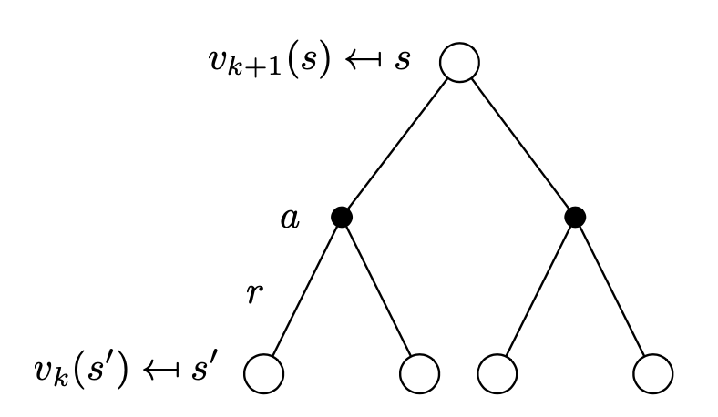
Consider a sequence of approximate value functions $v_0,v_1,\dots$, each mapping $\mathcal{S}^+\to\mathbb{R}$. Choosing $v_0$ arbitrarily (the terminal state, if any, must be given value 0). Using Bellman equation for $v_\pi$, we have an update rule:
\begin{align}
v_{k+1}(s)&\doteq\mathbb{E}_\pi\left[R_{t+1}+\gamma v_k(S_{k+1})\vert S_t=s\right] \\ &=\sum_a\pi(a|s)\sum_{s’,r}p(s’,r|s,a)\left[r+\gamma v_k(s’)\right]
\end{align}
for all $s\in\mathcal{S}$. Thanks to Banach’s fixed points theorem and as we have mentioned in that note, we have that the sequence $\{v_k\}\to v_\pi$ as $k\to\infty$. This algorithm is called iterative policy evaluation.
We have the backup diagram for this update.
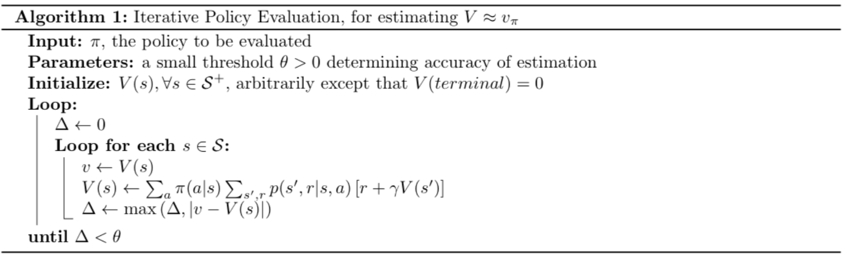
When implementing iterative policy evaluation method, for all $s\in\mathcal{S}$, we can use:
- One array to store the value functions, and update them "in-place" (asynchronous DP) \begin{equation} \color{red}{v(s)}\leftarrow\sum_a\pi(a|s)\sum_{s',r}p(s',r|s,a)\left[r+\color{red}{v(s')}\right] \end{equation}
- Two arrays in which the new value functions can be computed one by one from the old functions without the old ones being changed (synchronous DP) \begin{align} \color{red}{v_{new}(s)}&\leftarrow\sum_a\pi(a|s)\sum_{s',r}p(s',r|s,a)\left[r+\color{red}{v_{old}(s')}\right] \\ \color{red}{v_{old}}&\leftarrow\color{red}{v_{new}} \end{align}
Here is the pseudocode of the in-place iterative policy evaluation, given a policy $\pi$, for estimating $V\approx v_\pi$
Policy Improvement
The reason why we compute the value function for a given policy $\pi$ is to find better policies. Given the computed value function $v_\pi$ for an deterministic policy $\pi$, we already know how good it is for a state $s$ to choose action $a=\pi(s)$. Now what we are considering is, in $s$, if we instead take action $a\neq\pi$, will it be better?
In particular, in state $s$, selecting action $a$ and thereafter following the policy $\pi$, we have:
\begin{align}
q_\pi(s,a)&\doteq\mathbb{E}\left[R_{t+1}+\gamma v_\pi(S_{t+1})|S_t=s,A_t=a\right]\tag{2}\label{2} \\ &=\sum_{s’,r}p(s’,r|s,a)\left[r+\gamma v_\pi(s’)\right]
\end{align}
Theorem (Policy improvement theorem)
Let $\pi,\pi’$ be any pair of deterministic policies such that, for all $s\in\mathcal{S}$,
\begin{equation}
q_\pi(s,\pi’(s))\geq v_\pi(s)\tag{3}\label{3}
\end{equation}
Then $\pi’\geq\pi$, which means for all $s\in\mathcal{S}$, we have $v_{\pi’}(s)\geq v_\pi(s)$.
Proof
Deriving \eqref{3} combined with \eqref{2}, we have1:
\begin{align}
v_\pi(s)&\leq q_\pi(s,\pi’(s)) \\ &=\mathbb{E}\left[R_{t+1}+\gamma v_\pi(S_{t+1})|S_t=s,A_t=\pi’(s)\right]\tag{by \eqref{2}} \\ &=\mathbb{E}_{\pi’}\left[R_{t+1}+\gamma v_\pi(S_{t+1})|S_t=s\right] \\ &\leq\mathbb{E}_{\pi’}\left[R_{t+1}+\gamma q_\pi(S_{t+1},\pi’(S_{t+1}))|S_t=s\right]\tag{by \eqref{3}} \\ &=\mathbb{E}_{\pi’}\left[R_{t+1}+\gamma\mathbb{E}_{\pi’}\left[R_{t+2}+\gamma v_\pi(S_{t+2})|S_{t+1},A_{t+1}=\pi’(S_{t+1})\right]|S_t=s\right] \\ &=\mathbb{E}_{\pi’}\left[R_{t+1}+\gamma R_{t+2}+\gamma^2 v_\pi(S_{t+2})|S_t=s\right] \\ &\leq\mathbb{E}_{\pi’}\left[R_{t+1}+\gamma R_{t+2}+\gamma^2 R_{t+3}+\gamma^3 v_\pi(S_{t+3})|S_t=s\right] \\ &\quad\vdots \\ &\leq\mathbb{E}_{\pi’}\left[R_{t+1}+\gamma R_{t+2}+\gamma^2 R_{t+3}+\gamma^3 R_{t+4}+\dots|S_t=s\right] \\ &=v_{\pi’}(s)
\end{align}
Consider the new greedy policy, $\pi’$, which takes the action that looks best in the short term - after one step of lookahead - according to $v_\pi$, given by
\begin{align}
\pi’(s)&\doteq\underset{a}{\text{argmax}}\hspace{0.1cm}q_\pi(s,a) \\ &=\underset{a}{\text{argmax}}\hspace{0.1cm}\mathbb{E}\left[R_{t+1}+\gamma v_\pi(S_{t+1})|S_t=s,A_t=a\right]\tag{4}\label{4} \\ &=\underset{a}{\text{argmax}}\hspace{0.1cm}\sum_{s’,r}p(s’,r|s,a)\left[r+\gamma v_\pi(s’)\right]
\end{align}
By the above theorem, we have that the greedy policy is as good as, or better than, the original policy.
Suppose the new greedy policy, $\pi’$, is as good as, but not better than, $\pi$. Or in other words, $v_\pi=v_{\pi’}$. And from \eqref{4}, we have for all $s\in\mathcal{S}$,
\begin{align}
v_{\pi’}(s)&=\max_a\mathbb{E}\left[R_{t+1}+\gamma v_{\pi’}(S_{t+1})|S_t=s,A_t=a\right] \\ &=\max_a\sum_{s’,r}p(s’,r|s,a)\left[r+\gamma v_{\pi’}(s’)\right]
\end{align}
which is the Bellman optimality equation for action-value function. And therefore, $v_{\pi’}$ must be $v_*$. Hence, policy improvement must give us a strictly better policy except when the original one is already optimal2.
Policy Iteration
Once we have obtained a better policy, $\pi’$, by improving a policy $\pi$ using $v_\pi$, we can repeat the same process by computing $v_{\pi’}$, and improve it to yield an even better $\pi’’$. Repeating it again and again, we get an iterative procedure to improve the policy \begin{equation} \pi_0\xrightarrow[]{\text{evaluation}}v_{\pi_0}\xrightarrow[]{\text{improvement}}\pi_1\xrightarrow[]{\text{evaluation}}v_{\pi_1}\xrightarrow[]{\text{improvement}}\pi_2\xrightarrow[]{\text{evaluation}}\dots\xrightarrow[]{\text{improvement}}\pi_*\xrightarrow[]{\text{evaluation}}v_* \end{equation} Each following policy is a strictly improved version of the previous one (unless it is already optimal). Because a finite MDP has only a finite number of policies, this process must converge to an optimal policy and optimal value function in a finite number of iterations. This algorithm is called policy iteration. And here is the pseudocode of the policy iteration.
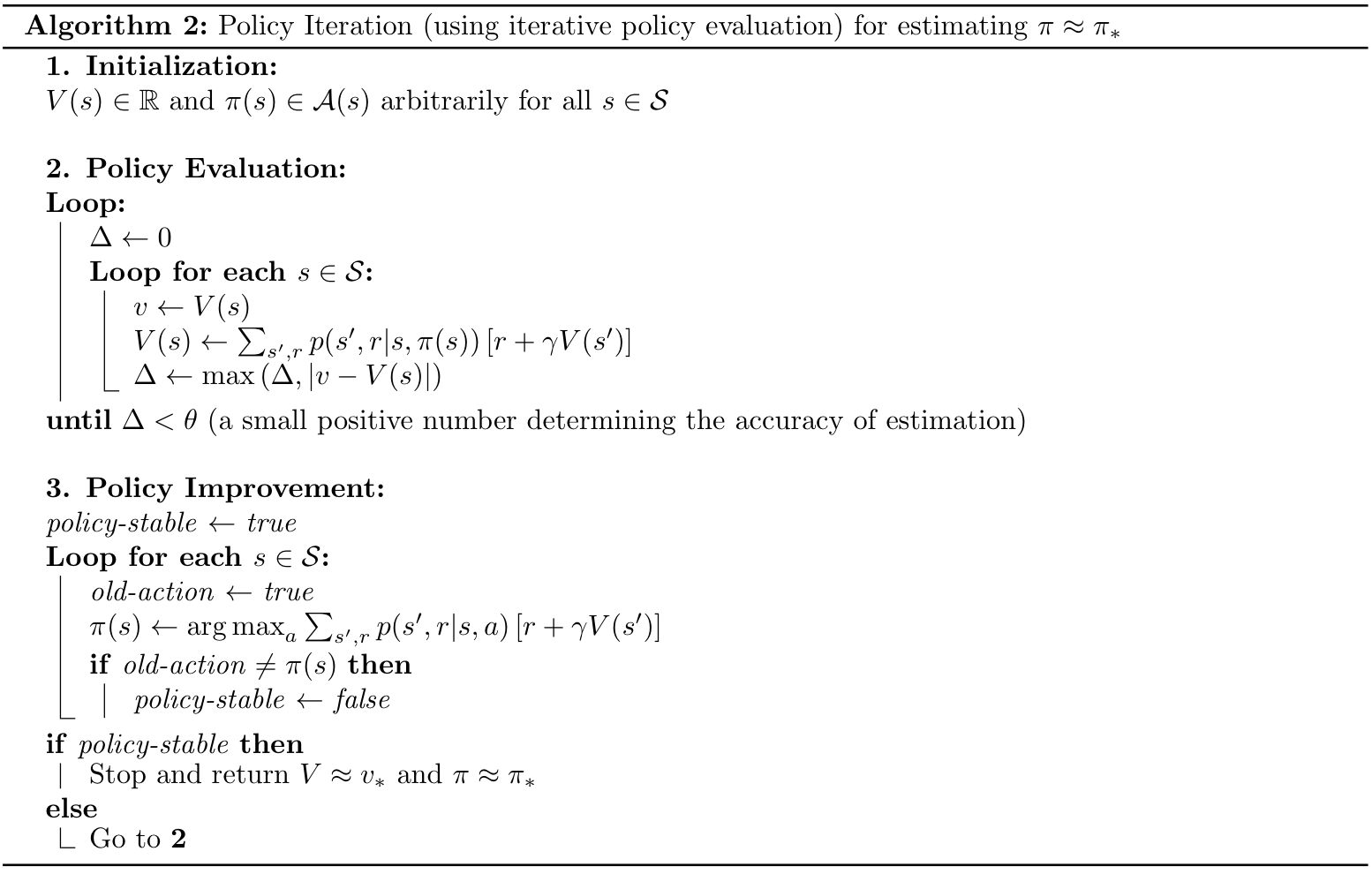
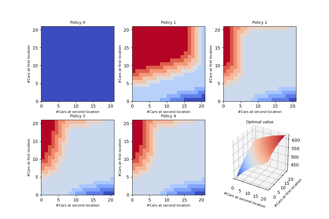
An example of using policy iteration on the Jack’s rental problem (RL book - example 4.2)
Value Iteration
When using policy iteration, each of its iterations involves policy evaluation, which requires multiple sweeps through the state set, and thus affects the computation performance.
Policy evaluation step of policy iteration, in fact, can be truncated in several ways without losing the convergence guarantees of policy iteration. One important special case is when policy evaluation is stopped after just one sweep (one update of each state). This algorithm is called value iteration, which follows this update:
\begin{align}
v_{k+1}&\doteq\max_a\mathbb{E}\left[R_{t+1}+\gamma v_k(S_{t+1})|S_t=s,A_t=a\right] \\ &=\max_a\sum_{s’,r}p(s’,r|s,a)\left[r+\gamma v_k(s’)\right],
\end{align}
for all $s\in\mathcal{S}$. Once again, thanks to Banach’s fixed point theorem, for an arbitrary $v_0$, we have that the sequence $\{v_k\}\to v_*$ as $k\to\infty$.
We have the backup diagram for this update3.
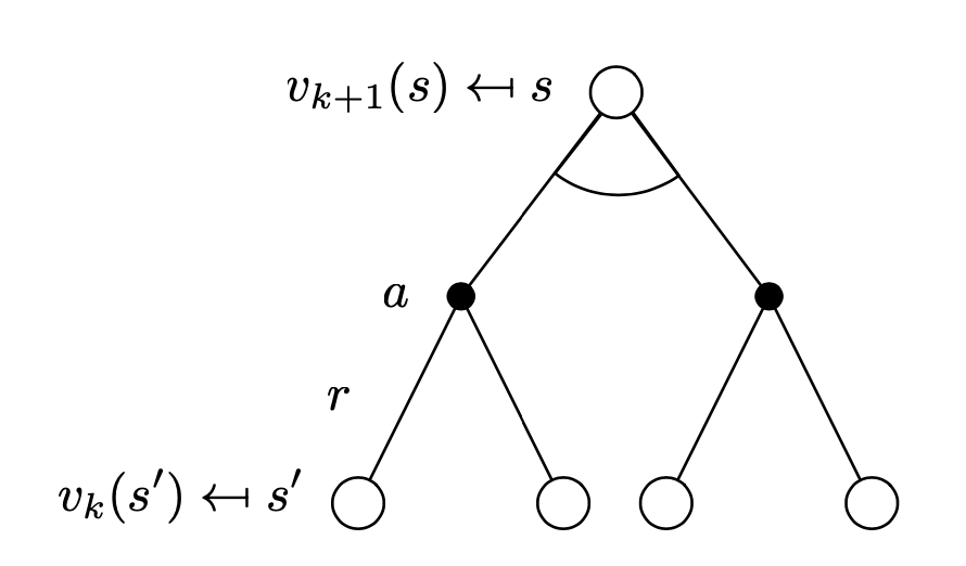
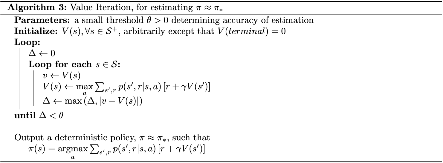
And here is the pseudocode of the value iteration.
Example - Gambler’s Problem
(This example is taken from RL book - example 4.3).
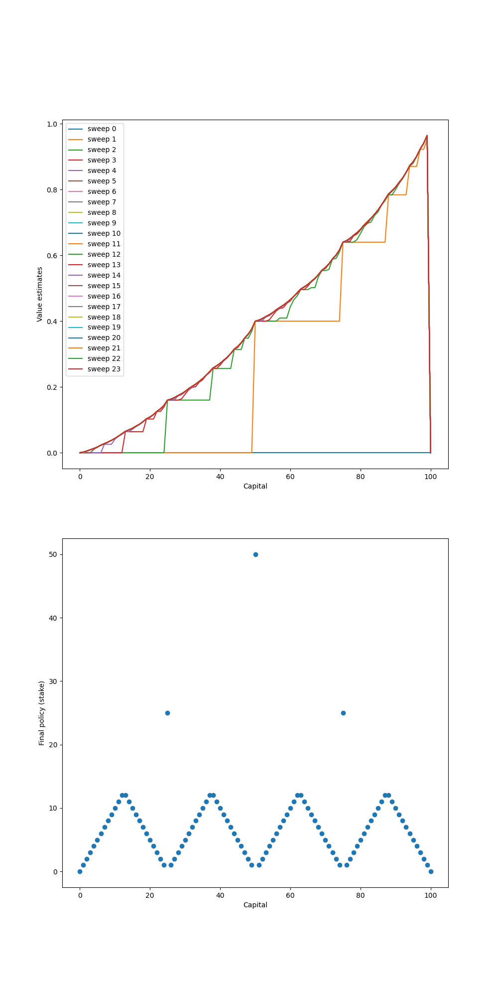
Let’s say you are a gambler, who decides to bet on the outcomes of sequence of coin flips. On each flip, you have to decide how many dollars, in integer, you will bet. Each time you win, when the coin comes up head, the amount of money you get is exactly the same as the money that you staked on that flip. Same it goes in the tail case, you will lose that amount of dollars. The game ends when you reach your goal, let’s assume, $\$100$, or when your hands are empty, $\$0$. This task can be formulated as undiscounted, episodic, finite MDP. The state is your capital, $s\in\{1,2,\dots,99\}$; the actions are stakes, $a\in\{0,1,\dots,\min\left(s,100-s\right)\}$. The reward is zero on all transitions except those on which you reach your goal, when it is $+1$. And we also assume that the probability of the coin coming up heads, $p_h=0.4$.
Solution code
The code can be found here.
import numpy as np
import matplotlib.pyplot as plt

GOAL = 100
#For convenience, we introduce 2 dummy states: 0 and terminal state
states = np.arange(0, GOAL + 1)
rewards = {'terminal': 1, 'non-terminal': 0}
HEAD_PROB = 0.4
GAMMA = 1  # discount factor


def value_iteration(theta):
    V = np.zeros(states.shape)
    V_set = []
    policy = np.zeros(V.shape)

    while True:
        delta = 0
        V_set.append(V.copy())
        for state in states[1:GOAL]:
            old_value = V[state].copy()

            actions = np.arange(0, min(state, GOAL - state) + 1)
            new_value = 0
            for action in actions:
                next_head_state = states[state] + action
                next_tail_state = states[state] - action
                head_reward = rewards['terminal'] if next_head_state == GOAL else rewards['non-terminal']
                tail_reward = rewards['non-terminal']
                value = HEAD_PROB * (head_reward + GAMMA * V[next_head_state]) + \
                    (1 - HEAD_PROB) * (tail_reward + GAMMA * V[next_tail_state])
                if value > new_value:
                    new_value = value

            V[state] = new_value
            delta = max(delta, abs(old_value - V[state]))
            print('Max value changed: ', delta)

        if delta < theta:
            V_set.append(V)
            break

    for state in states[1:GOAL]:
        values = []
        actions = np.arange(min(state, 100 - state) + 1)
        for action in actions:
            next_head_state = states[state] + action
            next_tail_state = states[state] - action
            head_reward = rewards['terminal'] if next_head_state == GOAL else rewards['non-terminal']
            tail_reward = rewards['non-terminal']
            values.append(HEAD_PROB * (head_reward + GAMMA * V[next_head_state]) +
                          (1 - HEAD_PROB) * (tail_reward + GAMMA * V[next_tail_state]))
        policy[state] = actions[np.argmax(np.round(values[1:], 4)) + 1]

    return V_set, policy


if __name__ == '__main__':
    theta = 1e-13
    value_funcs, optimal_policy = value_iteration(theta)
    optimal_value = value_funcs[-1]
    print(optimal_value)

    plt.figure(figsize=(10, 20))
    plt.subplot(211)
    for sweep, value in enumerate(value_funcs):
        plt.plot(value, label='sweep {}'.format(sweep))
    plt.xlabel('Capital')
    plt.ylabel('Value estimates')
    plt.legend(loc='best')
    plt.subplot(212)
    plt.scatter(states, optimal_policy)
    plt.xlabel('Capital')
    plt.ylabel('Final policy (stake)')

    plt.savefig('./gambler.png')
    plt.close()
And here is our results after running the code
Generalized Policy Iteration
The Generalized Policy Iteration (GPI) algorithm refers to the idea of combining policy evaluation and policy improvement together to improve the original policy.
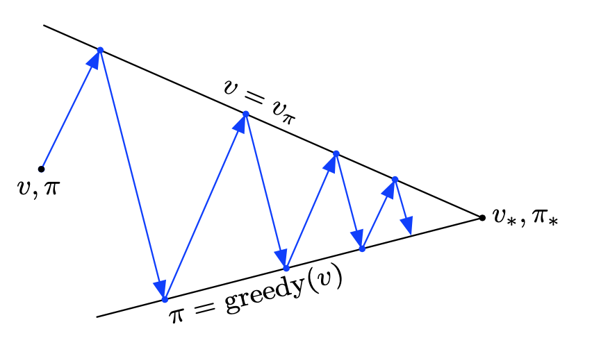
In GPI, the value function is repeatedly driven toward the true value of the current policy and at the same time the policy is being improved optimality with respect to its value function, as in the following diagram.
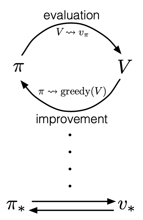
Once it reaches the stationary state (when both evaluation and improvement no long produce any updates), then the current value function and policy must be optimal.
The evaluation and improvement processes in GPI can be viewed as both competing and cooperating. They competing in the sense that on the one hand, making policy greedy w.r.t the value function typically makes value function incorrect for the new policy. And on the other hand, approximating the value function closer to the true value of the policy typically forces the policy is no longer to be greedy. But in the long run, they two processes cooperate to find a single joint solution: the optimal value function and an optimal policy.
References
[1] Richard S. Sutton & Andrew G. Barto. Reinforcement Learning: An Introduction. MIT press, 2018.
[2] David Silver. UCL course on RL.
[3] Csaba Szepesvári. Algorithms for Reinforcement Learning.
[4] A. Lazaric. Markov Decision Processes and Dynamic Programming.
[5] Wikipedia. Dynamic Programming.
[6] Shangtong Zhang. Reinforcement Learning: An Introduction implementation. Github.
[7] Policy Improvement theorem.
Footnotes
In the third step, the expression \begin{equation} \mathbb{E}_{\pi’}\left[R_{t+1}+\gamma v_\pi(S_{t+1})|S_t=s\right] \end{equation} means ‘’the discounted expected value when starting in state $s$, choosing action according to $\pi’$ for the next time step, and following $\pi$ thereafter". And so on for the two, or n next steps. Therefore, we have that: \begin{equation} \mathbb{E}_{\pi’}\left[R_{t+1}+\gamma v_\pi(S_{t+1})|S_t=s\right]=\mathbb{E}\left[R_{t+1}+\gamma v_\pi(S_{t+1})|S_t=s,A_t=\pi’(s)\right] \end{equation} ↩︎
The idea of policy improvement also extends to stochastic policies. ↩︎
Value iteration can be used in conjunction with action-value function, which takes the following update: \begin{align} q_{k+1}(s,a)&\doteq\mathbb{E}\left[R_{t+1}+\gamma\max_{a’}q_k(S_{t+1},a’)|S_t=s,A_t=a\right] \\ &=\sum_{s’,r}p(s’,r|s,a)\left[r+\gamma\max_{a’}q_k(s’,a’)\right] \end{align} Yep, that’s right, the sequence $\{q_k\}\to q_*$ as $k\to\infty$ at a geometric rate thanks to Banach’s fixed point theorem. ↩︎