Deep Q-learning

Notes on DQN and its variants.

Q-value iteration

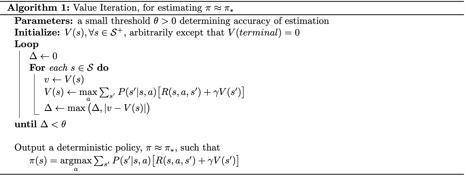
Recall that in the note Markov Decision Processes, Bellman equations, we have defined the state-value function for a policy $\pi$ to measure how good the state $s$ is, given as \begin{equation} V_\pi(s)=\sum_{a}\pi(a\vert s)\sum_{s’}P(s’\vert s,a)\big[R(s,a,s’)+\gamma V_\pi(s’)\big] \end{equation} From the definition of $V_\pi(s)$, we have continued to define the Bellman equation for the optimal value at state $s$, denoted $V^*(s)$: \begin{equation} V^*(s)=\max_{a}\sum_{s’}P(s’\vert s,a)\big[R(s,a,s’)+\gamma V^*(s’)\big],\label{eq:qvi.1} \end{equation} which characterizes the optimal value of state $s$ in terms of the optimal values of successor state $s’$.

Then, with Dynamic programming, we can solve \eqref{eq:qvi.1} by an iterative method, called value iteration, given as \begin{equation} V_{t+1}(s)=\max_{a}\sum_{s’}P(s’\vert s,a)\big[R(s,a,s’)+\gamma V_t(s’)\big]\hspace{1cm}\forall s\in\mathcal{S} \end{equation} For an arbitrary initial $V_0(s)$, the iteration, or the sequence $\{V_t\}$, will eventually converge to the optimal value function $V^*(s)$. This can be shown by applying the Banach’s fixed-point theorem, the one we have also used to prove the existence of the optimal policy, to prove that the iteration from $V_t(s)$ to $V_{t+1}(s)$ is a contraction mapping.

Details for value iteration method can be seen in the following pseudocode.

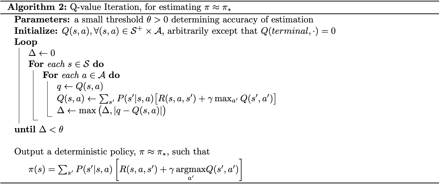
Remember that along with the state-value function $V_\pi(s)$, we have also defined the action-value function, or Q-values for a policy $\pi$, denoted $Q$, given by \begin{align} Q_\pi(s,a)&=\sum_{s’}P(s’\vert s,a)\left[R(s,a,s’)+\gamma\sum_{a’}\pi(a’\vert s’)Q_\pi(s’,a’)\right] \\ &=\sum_{s’}P(s’\vert s,a)\big[R(s,a,s’)+\gamma V_\pi(s’)\big] \end{align} which measures how good it is to be in state $s$ and take action $a$.

Analogously, we also have the Bellman equation for the optimal action-value function, given as \begin{align} Q^*(s,a)&=\sum_{s’}P(s’\vert s,a)\left[R(s,a,s’)+\gamma\max_{a’}Q^*(s’,a’)\right]\label{eq:qvi.2} \\ &=\sum_{s’}P(s’\vert s,a)\big[R(s,a,s’)+\gamma V^*(s’)\big]\label{eq:qvi.3} \end{align} The optimal value $Q^*(s,a)$ gives us the expected discounted cumulative reward for executing action $a$ at state $s$ and following the optimal policy, $\pi^*$, thereafter.

Equation \eqref{eq:qvi.3} allows us to write \begin{equation} V^*(s)=\max_a Q^*(s,a) \end{equation} Hence, analogy to the state-value function, we can also apply Dynamic programming to develop an iterative method in order to solve \eqref{eq:qvi.2}, called Q-value iteration. The method is given by the update rule \begin{equation} Q_{t+1}(s,a)=\sum_{s’}P(s’\vert s,a)\left[R(s,a,s’)+\gamma\max_{a’}Q_t(s’,a’)\right]\label{eq:qvi.4} \end{equation} This iteration, given an initial value $Q_0(s,a)$, eventually will also converge to the optimal Q-values $Q^*(s,a)$ due to the relationship between $V$ and $Q$ as defined above. Pseudocode for Q-value iteration is given below.

Q-learning

The update formula \eqref{eq:qvi.4} can be rewritten as an expected update \begin{equation} Q_{t+1}(s,a)=\mathbb{E}_{s’\sim P(s’\vert s,a)}\left[R(s,a,s’)+\gamma\max_{a’}Q_t(s’,a’)\right]\label{eq:ql.1} \end{equation} It is noticeable that the above update rule requires the transition model $P(s’\vert s,a)$. And since sample mean is an unbiased estimator of the population mean, or in other words, the expectation in \eqref{eq:ql.1} can be approximated by sampling, as

• At a state, taking (sampling) action $a$ (e.g. due to an $\varepsilon$-greedy policy), we get the next state: \begin{equation} s'\sim P(s'\vert s,a) \end{equation}
• Consider the old estimate $Q_t(s,a)$.
• Consider the new sample estimate (target): \begin{equation} Q_\text{target}=R(s,a,s')+\gamma\max_{a'}Q_t(s',a')\label{eq:ql.2} \end{equation}
• Append the new estimate into a running average to iteratively update Q-values: \begin{align} Q_{t+1}(s,a)&=(1-\alpha)Q_t(s,a)+\alpha Q_\text{target} \\ &=(1-\alpha)Q_t(s,a)+\alpha\left[R(s,a,s')+\gamma\max_{a'}Q_t(s',a')\right] \end{align}

This update rule is in form of a stochastic process, and thus, is guaranteed to converge to the optimal $Q^*$, under the stochastic approximation conditions for the learning rate $\alpha$. \begin{equation} \sum_{t=1}^{\infty}\alpha_t(s,a)=\infty\hspace{1cm}\text{and}\hspace{1cm}\sum_{t=1}^{\infty}\alpha_t^2(s,a)<\infty,\label{eq:ql.3} \end{equation} for all $(s,a)\in\mathcal{S}\times\mathcal{A}$.

The method is so called Q-learning, with pseudocode given below.

Neural networks with Q-learning

As a tabular method, Q-learning will work with a small and finite state-action pair space. However, for continuous environments, the exact solution might never be found. To overcome this, we have been instead trying to find an approximated solution.

In particular, we have tried to find an approximated action-value function $Q_\boldsymbol{\theta}(s,a)$, parameterized by a learnable vector $\boldsymbol{\theta}$, of the action-value function $Q(s,a)$, as \begin{equation} Q_\boldsymbol{\theta}(s,a) \end{equation} Then, we could have applied stochastic gradient descent (SGD) to repeatedly update $\boldsymbol{\theta}$ so as to minimize the loss function \begin{equation} L(\boldsymbol{\theta})=\mathbb{E}_{s,a\sim\mu(\cdot)}\Big[\big(Q(s,a)-Q_\boldsymbol{\theta}(s,a)\big)^2\Big] \end{equation} The resulting SGD update had the form \begin{align} \boldsymbol{\theta}_{t+1}&=\boldsymbol{\theta}_t-\frac{1}{2}\alpha\nabla_\boldsymbol{\theta}\big[Q(s_t,a_t)-Q_\boldsymbol{\theta}(s_t,a_t)\big]^2 \\ &=\boldsymbol{\theta}_t+\alpha\big[Q(s_t,a_t)-Q_\boldsymbol{\theta}(s_t,a_t)\big]\nabla_\boldsymbol{\theta}Q_\boldsymbol{\theta}(s_t,a_t)\label{eq:nql.1} \end{align} However, we could not perform the exact update \eqref{eq:nql.1} since the true value $Q(s_t,a_t)$ was unknown. Fortunately, we could instead replace it by $y_t$, which can be any approximation of $Q(s_t,a_t)$¹: \begin{equation} \boldsymbol{\theta}_{t+1}=\boldsymbol{\theta}_t+\alpha\big[y_t-Q_{\boldsymbol{\theta}_t}(s_t,a_t)\big]\nabla_\boldsymbol{\theta}Q_\boldsymbol{\theta}(s_t,a_t)\label{eq:nql.2} \end{equation}

Linear function approximation

Recall that, we have applied linear methods as our function approximators: \begin{equation} Q_\boldsymbol{\theta}(s,a)=\boldsymbol{\theta}^\text{T}\mathbf{f}(s,a), \end{equation} where $\mathbf{f}(s,a)$ represents the feature vector, (or basis functions) of the state-action pair $(s,a)$. Linear function approximation allowed us to rewrite \eqref{eq:nql.2} in a simplified form \begin{equation} \boldsymbol{\theta}_{t+1}=\boldsymbol{\theta}_t+\alpha\big[y_t-Q_{\boldsymbol{\theta}_t}(s_t,a_t)\big]\mathbf{f}(s_t,a_t)\label{eq:nql.3} \end{equation} The corresponding SGD method for Q-learning and Q-learning with linear function approximation are respectively given in form of \begin{equation} \boldsymbol{\theta}_{t+1}=\boldsymbol{\theta}_t+\alpha\left[R(s_t,a_t,s_{t+1})+\gamma\max_{a’}Q_{\boldsymbol{\theta}_t}(s_{t+1},a’)-Q_{\boldsymbol{\theta}_t}(s_t,a_t)\right]\nabla_\boldsymbol{\theta}Q_\boldsymbol{\theta}(s_t,a_t)\label{eq:nql.4} \end{equation} and \begin{equation} \boldsymbol{\theta}_{t+1}=\boldsymbol{\theta}_t+\alpha\left[R(s_t,a_t,s_{t+1})+\gamma\max_{a’}Q_{\boldsymbol{\theta}_t}(s_{t+1},a’)-Q_{\boldsymbol{\theta}_t}(s_t,a_t)\right]\mathbf{f}(s_t,a_t),\label{eq:nql.5} \end{equation} which both replace the $Q_\text{target}$ in \eqref{eq:ql.2} by the one parameterized by $\boldsymbol{\theta}$ \begin{equation} y_t=R(s_t,a_t,s_{t+1})+\gamma\max_{a’}Q_{\boldsymbol{\theta}_t}(s_{t+1},a’) \end{equation} However, in updating $\boldsymbol{\theta}_ {t+1}$, these methods both use the bootstrapping target: \begin{equation} R(s_t,a_t,s_{t+1})+\gamma\max_{a’}Q_{\boldsymbol{\theta}_t}(s_{t+1},a’), \end{equation} which depends on the current value $\boldsymbol{\theta}_t$, and thus will be biased. As a consequence, \eqref{eq:nql.4} does not guarantee to converge².

Such methods are known as semi-gradient since they take into account the effect of changing the weight vector $\boldsymbol{\theta}_t$ on the estimate, but ignore its effect on the target.

Deep Q-learning

On the other hands, we have already known that a neural network with particular settings for hidden layers and activation functions can approximate any continuous functions on a compact subsets of $\mathbb{R}^n$, so how about using it with the Q-learning algorithm?

Specifically, we will be using neural network with weight $\boldsymbol{\theta}$ as a function approximator for Q-learning update. The network is referred as Q-network, as the whole algorithm is so-called Deep Q-learning, and the agent is known as DQN in short for Deep Q-network.

The Q-network can be trained by minimizing a sequence of loss function $L_t(\boldsymbol{\theta}_t)$ that changes at each iteration $t$: \begin{equation} L_t(\boldsymbol{\theta}_t)=\mathbb{E}_{s,a\sim\rho(\cdot)}\Big[\big(y_t-Q_{\boldsymbol{\theta}_t}(s,a)\big)^2\Big],\label{eq:dqn.1} \end{equation} where \begin{equation} y_t=\mathbb{E}_{s’\sim\mathcal{E}}\left[R(s,a,s’)+\gamma\max_{a’}Q_{\boldsymbol{\theta}_{t-1}}(s’,a’)\vert s,a\right] \end{equation} is the target in iteration $t$, which follows as in \eqref{eq:nql.3}; and where $\rho(s,a)$ is referred as the behavior policy.

The TD target $y_t$ can approximated as \begin{equation} y_t=R(s_t,a_t,s_{t+1})+\max_{a’}Q_{\boldsymbol{\theta}_t}(s_{t+1},a’) \end{equation} To stabilize learning, DQN applies the following mechanisms.

Experience replay

Along with Q-network, the authors of deep-Q learning also introduce a technique called experience replay, which utilizes data efficiency and at the same time reduces the variance of the updates.

In particular, at each time step $t$, the experience, $e_t$, defined as \begin{equation} e_t=(s_t,a_t,r_t,s_{t+1}) \end{equation} is added into a set $\mathcal{D}$ of size $N$, which is sampled uniformly at the training time to apply Q-learning updates. This method provides some advantages:

• Each experience $e_t$ can be used in many weight updates.
• Uniformly sampling from $\mathcal{D}$ cancels out the correlations between consecutive experiences, i.e. $e_t, e_{t+1}$.

Target network

DQN introduces a target network $\hat{Q}$ parameterized by $\boldsymbol{\theta}^-$to generate the TD target $y_t$ in \eqref{eq:dqn.1} as \begin{equation} y_t=R(s_t,a_t,s_{t+1})+\gamma\max_{a’}\hat{Q}_{\boldsymbol{\theta}_t^-}(s_{t+1},a’)\label{eq:tn.1} \end{equation} The target network $\hat{Q}$ is cloned from $Q$ every $C$ Q-learning update steps, i.e. $\boldsymbol{\theta}^-\leftarrow\boldsymbol{\theta}$.

Improved variants

Double deep Q-learning

As stated before that the Q-learning method could lead to over optimistic value estimates. Moreover, Q-learning with function approximation, such as DQN, has also been proved to induce maximization bias. These results are due to that in Q-learning and DQN, the $\max$ operator uses the same values to both select and evaluate an action.

To reduce the overoptimism effect due to overestimation in DQN, we use a double estimator version of deep Q-learning, called Double Deep-Q learning, as we have used double Q-learning to mitigate the maximization bias in Q-learning.

The double DQN agent is similar to DQN, except that it replaces the target \eqref{eq:tn.1}, which can be rewritten as: \begin{equation} y_t=R(s_t,a_t,s_{t+1})+\gamma\hat{Q}_{\boldsymbol{\theta}_t^-}\left(s_{t+1},\underset{a}{\text{argmax}}\hspace{0.1cm}\hat{Q}_{\boldsymbol{\theta}_t^-}(s_{t+1},a)\right), \end{equation} with \begin{equation} y_t=R(s_t,a_t,s_{t+1})+\gamma\hat{Q}_{\boldsymbol{\theta}_t^-}\left(s_{t+1},\underset{a}{\text{argmax}}\hspace{0.1cm}Q_{\boldsymbol{\theta}_t}(s_{t+1},a)\right) \end{equation}

Prioritized replay

Dueling network

Rainbow

References

[1] Tommi Jaakkola, Michael I. Jordan, Satinder P. Singh. On the Convergence of Stochastic Iterative Dynamic Programming Algorithms. A.I. Memo No. 1441, 1993.

[2] Richard S. Sutton & Andrew G. Barto. Reinforcement Learning: An Introduction. MIT press, 2018.

[3] Pieter Abbeel. Foundations of Deep RL Series, YouTube, 2021.

[4] Vlad Mnih, et al. Playing Atari with Deep Reinforcement Learning, 2013.

[5] Vlad Mnih, et al. Human Level Control Through Deep Reinforcement Learning. Nature, 2015.

[6] Hado van Hasselt, Arthur Guez, David Silver. Deep Reinforcement Learning with Double Q-learning. AAAI16, 2016.

[7] Ziyu Wang, Tom Schaul, Matteo Hessel, Hado van Hasselt, Marc Lanctot, Nando de Freitas. Dueling Network Architectures for Deep Reinforcement Learning. arXiv:1511.06581, 2015.

[8] Tom Schaul, John Quan, Ioannis Antonoglou, David Silver. Prioritized Experience Replay. arXiv:1511.05952, 2016.

[9] Taisuke Kobayashi, Wendyam Eric Lionel Ilboudo. t-Soft Update of Target Network for Deep Reinforcement Learning. arXiv:2008.10861, 2020.

[10] Zhikang T. Wang, Masahito Ueda. Convergent and Efficient Deep Q Network Algorithm. arXiv:2106.15419, 2022.

Footnotes