AlphaZero

AlphaGo

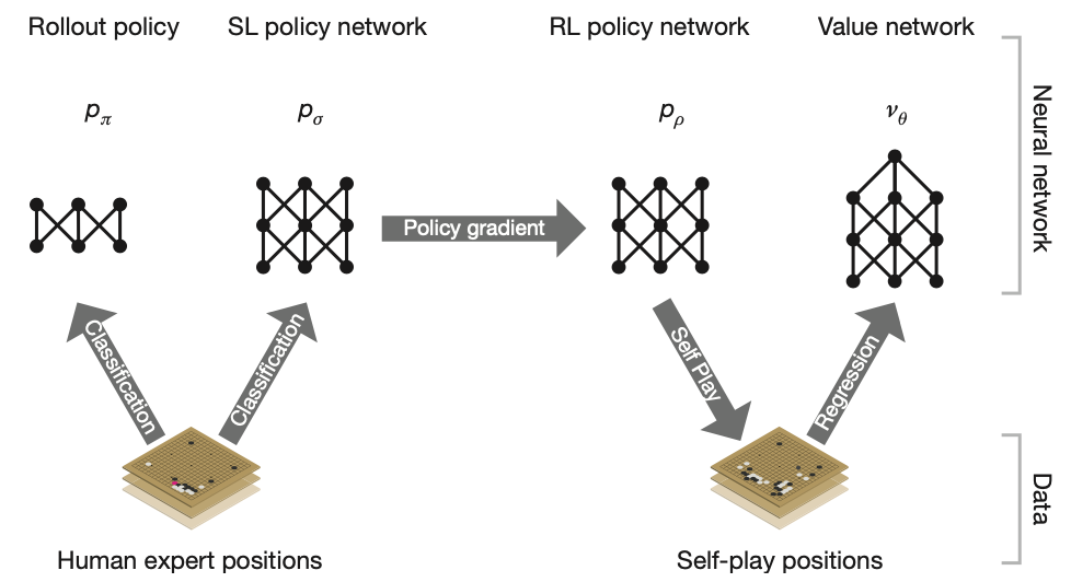
The training pipeline used in AlphaGo can be divided into following stages:

• Using a dataset of human experts positions, a supervised learning (SL) policy network $p_\sigma$ and, a rollout policy $p_\pi$, which can sample actions rapidly, are trained by classification to predict player moves.
• Initializing with the SL policy network $p_\sigma$, it uses policy gradient to train a reinforcement learning (RL) policy network $p_\rho$ with the goal to maximize the winning outcome against previous versions of the policy network. This process generates a dataset of self-play games.
• Via the dataset of self-play moves, a value network $v_\theta$ is trained by regression to predict the expected outcome (win or lose).

SL policy network $p_\sigma$, rollout network $p_\pi$

The policy network $p_\sigma(a\vert s)$ takes as its input a simple representation of the board state $s$ and outputs a probability distribution over all legal moves $a$. The network is trained to maximize the likelihood of the human move $a$ selected in state $s$ by using SGA \begin{equation} \Delta\sigma\propto\frac{\partial\log p_\sigma(a\vert s)}{\partial\sigma} \end{equation} The rollout network $p_\pi(a\vert s)$ is trained using a linear softmax of small pattern features. This network is less accurate but faster selecting action than $p_\sigma$.

RL policy network $p_\rho$

The RL policy network $p_\rho$ has the same architecture as $p_\sigma$ and its weights are also initialized at $\rho=\sigma$.

The games are between the current policy $p_\rho$ and a randomly selected previous iteration $p_{\rho^-}$ of its, which prevents overfitting to the current policy. The outcome $z_t=\pm r(s_T)$ of each game is the terminal reward at the end of the game from the perspective, where $r(s)$ is the reward function which is zero for all non-terminal step $t<T$, i.e. $z_t=+1$ for winning and $-1$ for losing.

The weights $\rho$ are updated by SGA in the direction that maximizes expected outcome \begin{equation} \Delta\rho\propto\frac{\partial\log p_\rho(a_t\vert s_t)}{\partial\rho}z_t \end{equation}

Value network $v_\theta$

For each RL policy network $p$, we define its corresponding value function to be \begin{equation} v^{p}(s)=\mathbb{E}\big[z_t\vert s_t=s,a_{t\ldots T}\sim p\big] \end{equation} Ideally, we wish for the optimal policy $p^*$ with value function $v^*$. In tabular problem, this can be done via dynamic programming. However, in large state space problem like Go, we instead use an estimation of $v^{p_\rho}$. Specifically, we approximate the value function using a value network $v_\theta(s)$ parameterized by $\theta$, $v_\theta(s)\approx v^{p_\rho}(s)\approx v^*(s)$.

This network has a similar structure to the policy network $p_\rho$, but outputs a scalar value instead of a probability distribution. The weights $\theta$ is updated via SGD in the direction that minimizes the MSE between the predicted value $v_\theta(s)$ and the corresponding outcome $z$ by using regression on state-outcome pair $(s,z)$¹ \begin{equation} \Delta\theta\propto\frac{\partial v_\theta(s)}{\partial\theta}(z-v_\theta(s)) \end{equation}

Searching with policy and value networks

Once trained, the policy network $p_\rho$ and value network $v_\theta$ then are combined with a Monte Carlo tree search (MCTS) to provide a lookahead search.

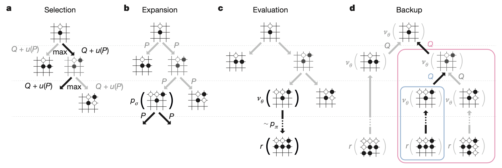
Each node $s$ in the search tree contains edges $(s,a)$ for all legal action $a\in\mathcal{A}(s)$. Each edge $(s,a)$ stores a set of statistics \begin{equation} \{P(s,a),N_v(s,a),N_r(s,a),W_v(s,a),W_r(s,a),Q(s,a)\} \end{equation} where $P(s,a)$ is the prior probability, $W_v(s,a),W_r(s,a)$ are Monte Carlo estimates of total action value, accumulated over $N_v(s,a)$ leaf evaluations and $N_r(s,a)$ rollout rewards, respectively, and $Q(s,a)$ is the combined mean action value for that edge. The algorithm proceeds by iterating over four phases.

• Selection. The stage begin at the root node $s_0$ of the tree and finishes when the simulation reaches a leaf node $s_L$ at time-step $L$. At each of these time-steps $t< L$, an action $a_t$ is that maximizes the UCB score is selected \begin{align} a_t&=\underset{a}{\text{argmax}}(Q(s_t,a)+u(s_t,a)) \\ u(s,a)&=c_\text{puct}\frac{\sqrt{\sum_b N_r(s,b)}}{1+N_r(s,a)}, \end{align} where $c_\text{puct}$ is the constant that controls the level of exploration.
• Expansion. When the visit count exceeds a threshold, $N_r(s,a)>n_\text{thr}$, the successor state $s'$ is added to the search tree with statistics initialized using a tree policy $p_\tau(a\vert s')$ (similar to the rollout policy but with more features). \begin{equation} \{N(s',a)=N_r(s',a)=0,W(s',a)=W_r(s',a)=0,P(s',a)=p_\sigma(a\vert s')\} \end{equation}
• Evaluation. The leaf $s_L$ is added to the queue for evaluation $v_\theta(s_L)$ by the value network, unless if has been evaluated before.
  The second rollout phase of each simulation begin at leaf node $s_L$ and continue until the end of the game. At each of these time-step $t\geq L$, actions are selected by both players according to the rollout policy, $a_t\sim p_\pi(\cdot\vert s_t)$.
  When the game reaches a terminal state, the outcome $z_t=\pm r(s_T)$ is computed from the final score.
• Backup. At each step $t\leq L$ of the simulation, the rollout statistics are updated as if it has lost $n_\text{vl}$ games \begin{align} N_r(s_t,a_t)&\leftarrow N_r(s_t,a_t)+n_\text{vl} \\ W_r(s_t,a_t)&\leftarrow W_r(s_t,a_t)-n_\text{vl} \end{align} This virtual loss discourages other threads from simultaneously exploring the identical variation.
  At the end of the simulation, the rollout statistics are updated a backward pass through each step $t\leq L$, replacing the virtual loss by the outcome \begin{align} N_r(s_t,a_t)&\leftarrow N_r(s_t,a_t)-n_\text{vl}+1 \\ W_r(s_t,a_t)&\leftarrow W_r(s_t,a_t)+n_\text{vl}+z_t \end{align} Asynchronously, a separate backward pass through each step $t\leq L$ is initiated when the evaluation of $s_L$ via $v_\theta$ completes \begin{align} N_v(s_t,a_t)&\leftarrow N_v(s_t,a_t)+1 \\ W_v(s_t,a_t)&\leftarrow W_v(s_t,a_t)+v_\theta(s_L) \end{align} The overall evaluation of each state action pair is a weighted average of the MC estimates \begin{equation} Q(s,a)=(1-\lambda)\frac{W_v(s,a)}{N_v(s,a)}+\lambda\frac{W_r(s,a)}{N_r(s,a)} \end{equation} where $\lambda$ is the weighting parameter.

AlphaGo Zero

AlphaGo Zero differs from its predecessor, AlphaGo, in various aspects:

• It is trained only via self-play reinforcement learning, starting from random play, without supervised.
• It uses only the black and white stones from the board as input features.
• It uses a single neural network, rather than separate policy and value networks.
• It uses a simpler tree search to evaluate positions and sample moves, without doing any MC rollouts.

The self-play training pipeline of AlphaGo Zero contains three main components, all executed asynchronously in parallel.

• Neural network parameters $\theta_i$ are continually optimized from recent self-play data.
• AlphaGo Zero player $\alpha_{\theta_i}$ are continually evaluated.
• The best performing player so far, $\alpha_{\theta_*}$, is used to generate new self-play data.

Neural network training

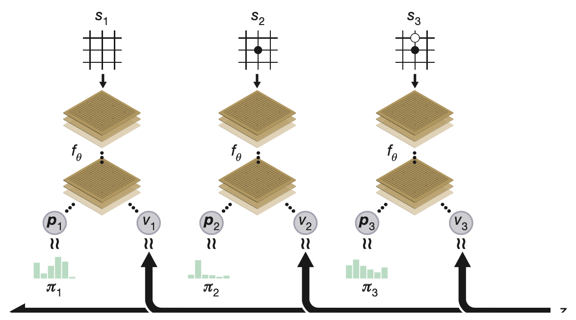
AlphaGo Zero utilizes a neural network $f_\theta$ parameterized by $\theta$. This network takes the board position $s$ as an input and outputs a vector of move probabilities $\mathbf{p}$ with components $p_a=Pr(a\vert s)$ for each action $a$ and a scalar value $v$ estimating the expected outcome $z$ of the game from position $s$, $v\approx\mathbb{E}\big[z\vert s\big]$ \begin{equation} (\mathbf{p},v)=f_\theta(s) \end{equation} The training of $f_\theta$ proceeds as

• The network is initialized to random weights $\theta_0$.
• At each subsequent iteration $i\geq 1$, games of self-play are generated.
• At each time-step $t$, an MCTS search $\boldsymbol{\pi}_t=\alpha_{\theta_{i-1}}(s_t)$ is executed using the previous iteration of neural network $f_{\theta_{i-1}}$ and a move is played by sampling from $\boldsymbol{\pi}_t$.
• A game terminates at step $T$ when the terminal condition is reached (both player pass, the search value drops below a resignation threshold or the game exceeds a maximum length), the game is then scored to give a final reward of $r_T\in\{-1,+1\}$.
• The data for each time-step $t$ is stored as $(s_t,\boldsymbol{\pi}_t,z_t)$ where $z_t=\pm r_T$ is the game winner from the perspective of the current player at step $t$.
  In the mean time, new network parameters $\theta_i$ are trained from data $(s,\boldsymbol{\pi},z)$ sampled uniformly among all time-steps of the last iteration of self-play.
• The neural network $(\mathbf{p},v)$ is adjusted to minimize the error between the predicted value $v$ and the self-play winner $z$ while concurrently maximize the similarity of $\mathbf{p}$ to the search probability $\boldsymbol{\pi}$. Specifically, the parameters $\theta$ is updated by gradient descent on a loss function $l$ that sums over the MSE and cross-entropy losses \begin{equation} l=(z-v)^2-\boldsymbol{\pi}^\text{T}\log\mathbf{p}+c\Vert\theta\Vert^2, \end{equation} where $c$ is the L2 weight regularization parameter.
• The optimization process of $f_\theta$ produces a checkpoint every number of training steps. Each checkpoint $f_{\theta_j}$ is evaluated by competing the performance of an MCTS $\alpha_{\theta_j}$, which uses $f_{\theta_j}$ to evaluate leaf positions and prior probabilities, with the current best $\alpha_{\theta_*}$, which uses $f_{\theta_*}$ to produce search probabilities.
  The replacement of $f_{\theta_*}$ by $f_{\theta_j}$ to generate next batch of self-play games occurs when $\alpha_{\theta_j}$ wins $\alpha_{\theta_*}$ by a margin of $55\%$.

Self-play algorithm

The self-play mechanism used by AlphaGo Zero proceeds as:

• The AlphaGo Zero agent plays a game $s_1,\ldots,s_T$ against itself.
• In each position $s_t$, an MCTS $\alpha_\theta$ is executed using the latest neural network $f_\theta$.
• Moves are selected according to the search probabilities outputed by the the MCTS, $a_t\sim\boldsymbol{\pi}_t$.
• The terminal position $s_T$ is scored according to the rules of the game to compute the game winner $z$.

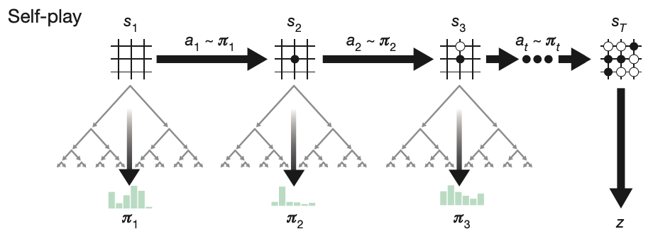
The self-play algorithm in AlphaGo Zero can be understood as a policy iteration procedure. Indeed, in each position $s$, an MCTS $\alpha_\theta$ is performed guided by the neural network $f_\theta$. The move probabilities $\boldsymbol{\pi}$ computed by $\alpha_\theta$ is usually much effective than the one, $\mathbf{p}$, produced by $f_\theta$ (i.e. selecting stronger moves). Thus, MCTS then can be observed as a policy improvement operator. Moreover, self-play with search, using the improved policy $\boldsymbol{\pi}$ to select move, then using the game winner $z$ as a sample of the value, might be observed as a policy evaluation operator.

The neural network’s parameters $\theta$ are updated to make the move probabilities and value $(\mathbf{p},v)$ more closely match the improved search probabilities and self-play winner $(\boldsymbol{\pi},z)$. These new parameters are used in the next iteration of self-play to make the search even stronger.

Search algorithm

Each node $s$ in the search tree contains edges $(s,a)$ for all legal action $a\in\mathcal{A}(s)$. Each edge $(s,a)$ stores a set of statistics \begin{equation} \{N(s,a),W(s,a),Q(s,a),P(s,a)\} \end{equation} where $N(s,a)$ is the visit count, $W(s,a)$ is the total action value, $Q(s,a)$ is the mean action value and $P(s,a)$ is the prior probability of selecting the edge. The algorithm iterates over three stages and then select an action to play.

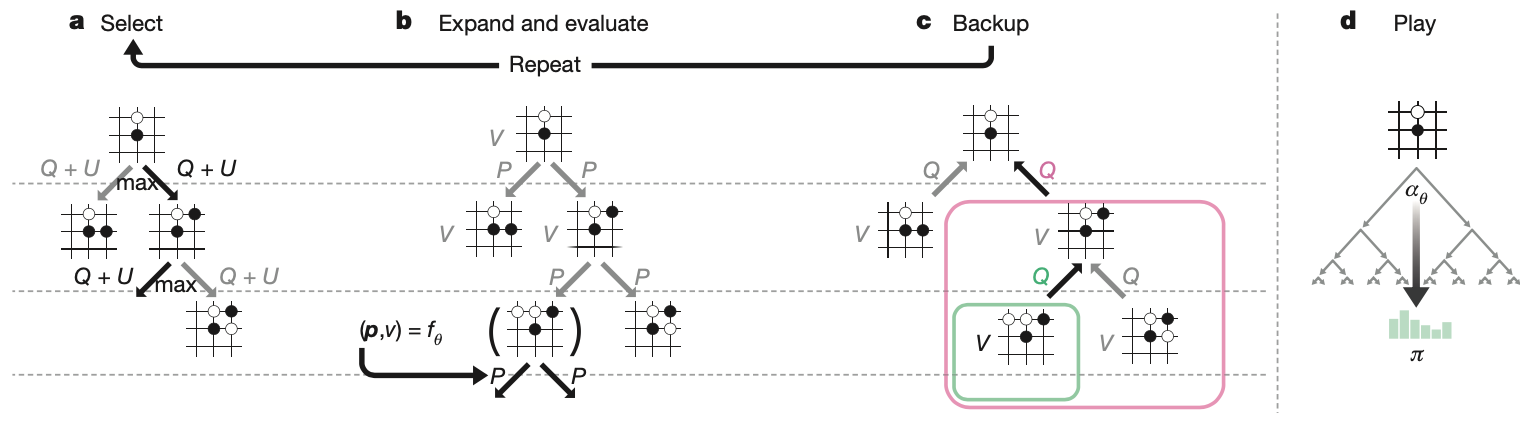
• Select. This stage is identical to the one in AlphaGo. The selection phase begins at the root node $s_0$ and finishes when the simulation reaches a leaf node $s_L$ at time-step $L$. At each of these time-step, $t< L$, an action $a_t$ that maximizes the UCB is selected \begin{align} a_t&=\underset{a}{\text{argmax}}(Q(s_t,a)+U(s_t,a)) \\ U(s,a)&=c_\text{puct}P(s,a)\frac{\sqrt{\sum_b N(s,b)}}{1+N(s,a)}, \end{align} where $c_\text{puct}$ is the UCT constant that controls the level exploration.
• Expand and evaluate. The leaf node $s_L$ is added to the queue for neural network evaluation \begin{equation} (d_i(\mathbf{p},v))=f_\theta(d_i(s_L)), \end{equation} where $d_i$ is a dihedral reflection or rotation selected uniformly for $i\in\{1,\ldots,8\}$. The leaf node is then expanded and each edge $(s_L,a)$ is initialized to \begin{equation} \{N(s_L,a)=0,W(s_L,a)=0,Q(s_L,a)=0,P(s_L,a)=p_a\}, \end{equation} and the value $v$ is then backed up.
• Backup. The edge statistics are updated in a backward pass through each step $t\leq L$. \begin{align} N(s_t,a_t)&\leftarrow N(s_t,a_t)+1 \\ W(s_t,a_t)&\leftarrow W(s_t,a_t)+v \\ Q(s_t,a_t)&\leftarrow\frac{W(s_t,a_t)}{N(s_t,a_t)} \end{align} Similar to AlphaGo, we also use virtual loss to ensure each thread evaluates different nodes.
• Play. At the end of the search, the best child node corresponding to a move $a$ is selected from \begin{equation} \pi(a\vert s_0)=\frac{N(s_0,a)^{1/\tau}}{\sum_b N(s_0,b)^{1/\tau}}, \end{equation} where $\tau$ is the temperature parameter that controls the level of exploration.

AlphaZero

AlphaZero is a more generic version of AlphaGo Zero. With the same algorithm and network architecture, the authors have successfully applied it to the game of chess and shogi, as well as Go. It has some respects differ from AlphaGo Zero:

• AlphaGo Zero estimated and optimized the probability of winning, using the fact that Go is a binary-outcome game (either win or loss). On the other hand, since drawn outcome can happen in a game of chess and shogi, and in fact the optimal strategy to chess is a draw, AlphaZero estimates and optimizes the expected outcome instead.
• The rules of Go are specifically invariant to rotation and reflection². AlphaGo Zero exploited this fact to augment the training data (generating eight symmetries for each raw board position) and transformed (by applying a randomly selected rotation or reflection operator) the board position during MCTS. Conversely, in order to generalize to a broader rules of games, AlphaZero does not augment the training data and also does not transform the board position during MCTS.
• In AlphaGo Zero, self-play games were generated by the best player from all previous iterations. After each iteration of training, the new player competed against the best player so far and replaced the best player if it won by a margin of $55\%$. On the contrary, AlphaZero only maintains single neural network that is updated continually rather than waiting for an iteration to complete. Self-play games are then always generated by using the latest parameters from this neural network.

References

[1] David Silver, Aja Huang, Chris J. Maddison et al. Mastering the game of Go with deep neural networks and tree search. Nature 529, 484–489, 2016.

[2] David Silver, Julian Schrittwieser, Karen Simonyan et al. Mastering the game of Go without human knowledge. Nature 550, 354–359, 2017.

[3] David Silver, Thomas Hubert, Julian Schrittwieser et al. A general reinforcement learning algorithm that masters chess, shogi, and Go through self-play. Science 362, 1140-1144, 2018.

[4] Richard S. Sutton & Andrew G. Barto. Reinforcement Learning: An Introduction. MIT press, 2018.

Footnotes