Gaussian Distribution & Gaussian Network Models

Notes on Gaussian distribution & Gaussian network models.

$\newcommand{\Var}{\mathrm{Var}}$ $\newcommand{\Cov}{\mathrm{Cov}}$

Normal Distribution

Standard Normal Distribution

A continuous random variable $Z$ is said to have the standard Normal distribution if its PDF $\varphi$ is given by \begin{equation} \varphi(z)=\frac{1}{\sqrt{2\pi}e^{-z^2/2}},\hspace{1cm}z\in(-\infty,\infty) \end{equation} and denoted $Z\sim\mathcal{N}(0,1)$, since, as we will show, $Z$ has mean $0$ and variance $1$. Before that, let us compute the CDF of $Z$, which is given as \begin{equation} \Phi(z)=\int_{-\infty}^{z}\varphi(t)dt=\int_{-\infty}^{z}\frac{1}{\sqrt{2\pi}}e^{-t^2/2}dt \end{equation} We continue by verifying that $\mathcal{N}{(0,1)}$ is indeed a distribution. Since $\varphi(z)\geq 0$, our problem remains to show that the PDF of $Z$ integrates to $1$. In particular, we have \begin{align} \left(\int_{-\infty}^{\infty}e^{-x^2/2}dx\right)\left(\int_{-\infty}^{\infty}e^{-y^2/2}dy\right)&=\int_{-\infty}^{\infty}\int_{-\infty}^{\infty}e^{-x^2/2}e^{-y^2/2}dydx \\ &=\int_{-\infty}^{\infty}\int_{-\infty}^{\infty}e^{-\frac{x^2+y^2}{2}}dxdy\label{eq:sn.1} \end{align} Let us change the variables, specifically, we will be changing from the Cartesian coordinate to the polar coordinate, by letting \begin{align} x&=r\cos\theta, \\ y&=r\sin\theta, \end{align} where $r\geq 0$ is the distance from $(x,y)$ to the origin and $\theta\in[0,2\pi)$ is the angle. The Jacobian matrix of this transformation is \begin{equation} \frac{d(x,y)}{d(r,\theta)}=\left[\begin{matrix}\cos\theta&-r\sin\theta \\ \sin\theta& r\cos\theta\end{matrix}\right], \end{equation} which implies that \begin{equation} \text{det}\frac{d(x,y)}{d(r,\theta)}=\text{det}\left[\begin{matrix}\cos\theta&-r\sin\theta \\ \sin\theta& r\cos\theta\end{matrix}\right]=1 \end{equation} This makes us continue to derive \eqref{eq:sn.1} as \begin{align} \int_{-\infty}^{\infty}\int_{-\infty}^{\infty}e^{-\frac{x^2+y^2}{2}}dxdy&=\int_{0}^{2\pi}\int_{0}^{\infty}e^{-r^2/2}\left\vert\text{det}\frac{d(x,y)}{d(r,\theta)}\right\vert rdrd\theta \\ &=\int_{0}^{2\pi}\int_{0}^{\infty}e^{-r^2/2}rdrd\theta \end{align} Let $u=r^2/2$, then $du=rdr$, we have \begin{equation} \int_{0}^{2\pi}\int_{0}^{\infty}e^{-r^2/2}rdrd\theta=\int_{0}^{2\pi}\int_{0}^{\infty}e^{-u}dud\theta=\int_{0}^{2\pi}1d\theta=2\pi \end{equation} And hence, we can conclude that \begin{equation} \int_{-\infty}^{\infty}e^{-z^2/2}dz=\sqrt{2\pi} \end{equation} or \begin{equation} \int_{-\infty}^{\infty}\varphi(z)dz=\int_{-\infty}^{\infty}\frac{1}{\sqrt{2\pi}}e^{-z^2/2}dz=1 \end{equation}

Standard Mean, Standard Variance

We have that the mean of a standard Normal r.v $Z$ is given as \begin{align} \mathbb{E}(Z)&=\int_{-\infty}^{\infty}\frac{1}{\sqrt{2\pi}}z e^{-z^2/2}dz \\ &=\frac{1}{\sqrt{2\pi}}\left(\int_{0}^{\infty}z e^{-z^2/2}dz+\int_{-\infty}^{0}z e^{-z^2/2}dz\right) \\ &=\frac{1}{\sqrt{2\pi}}\left(\int_{0}^{\infty}z e^{-z^2/2}dz-\int_{0}^{\infty}z e^{-z^2/2}dz\right) \\ &=0 \end{align} where in the third step, we use the fact that $ze^{-z^2/2}$ is an odd function.

Given the mean of $Z$, we have its variance is then can be computed by \begin{align} \Var(Z)&=\mathbb{E}(Z^2)-(\mathbb{E}Z)^2 \\ &=\mathbb{E}(Z^2) \\ &=\int_{-\infty}^{\infty}\frac{1}{\sqrt{2\pi}}z^2 e^{-z^2/2}dz \\ &=\frac{\sqrt{2}}{\sqrt{\pi}}\int_{0}^{\infty}z^2 e^{-z^2/2}dz \end{align} where the last step uses the fact that $z^2 e^{-z^2/2}$ is an even function. We continue by using integration by parts with $u=z$ and $dv=z e^{-z^2/2}$, then $du=dz$ and $v=-e^{-z^2/2}$. Thus, \begin{align} \Var(Z)&=\frac{\sqrt{2}}{\sqrt{\pi}}\left(-z e^{-z^2/2}\Big\vert_{0}^{\infty}+\int_{0}^{\infty}e^{-z^2/2}dz\right) \\ &=\frac{\sqrt{2}}{\sqrt{\pi}}\left(0+\frac{\sqrt{2\pi}}{2}\right) \\ &=1 \end{align}

Univariate Normal Distribution

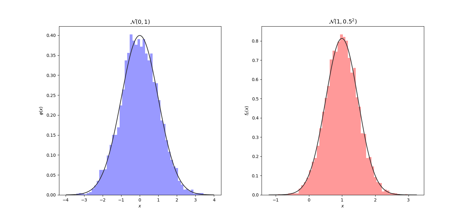
Let $Z\sim\mathcal{N}(0,1)$ be a standard Normal r.v, then a continuous r.v $X$ is said to be a Gaussian or to have the (Univariate) Normal distribution with mean $\mu$ and variance $\sigma^2$, denoted $X\sim\mathcal{N}(\mu,\sigma^2)$ if \begin{equation} X=\mu+\sigma Z \end{equation} The mean and variance of $X$ can be verified to be $\mu$ and $\sigma^2$ respectively easily by using the linearity of expectation and variance.

To derive the PDF formula for $X$, let us first start with its CDF, which is given by \begin{equation} P(X\leq x)=P\left(\frac{X-\mu}{\sigma}\leq\frac{x-\mu}{\sigma}\right)=P\left(Z\leq\frac{x-\mu}{\sigma}\right)=\Phi\left(\frac{x-\mu}{\sigma}\right) \end{equation} We then obtain the PDF of $X$ by differentiating its CDF \begin{align} p_X(x)&=\frac{d}{dx}\Phi\left(\frac{x-\mu}{\sigma}\right)=\frac{1}{\sigma}\varphi\left(\frac{x-\mu}{\sigma}\right) \\ &=\dfrac{1}{\sqrt{2\pi}\sigma}\exp\left(-\dfrac{(x-\mu)^2}{2\sigma^2}\right) \end{align}

Below are some illustrations of the Univariate Normal distribution.

Multivariate Normal Distribution

A $k$-dimensional random vector $\mathbf{X}=\left(X_1,\dots,X_D\right)^\text{T}$ is said to have a Multivariate Normal (MVN) distribution if every linear combination of the $X_i$ has a Normal distribution. Which means \begin{equation} t_1X_1+\ldots+t_DX_D \end{equation} is normally distributed for any choice of constants $t_1,\dots,t_D$. Distribution of $\mathbf{X}$ then can be written in the following notation \begin{equation} \mathbf{X}\sim\mathcal{N}(\boldsymbol{\mu},\boldsymbol{\Sigma}), \end{equation} where \begin{equation} \boldsymbol{\mu}=\mathbb{E}\mathbf{X}=\mathbb{E}\left(\mu_1,\ldots,\mu_k\right)^\text{T}=\left(\mathbb{E}X_1,\ldots,\mathbb{E}X_k\right)^\text{T} \end{equation} is the $D$-dimensional mean vector, and covariance matrix $\mathbf{\Sigma}\in\mathbb{R}^{D\times D}$ with \begin{equation} \boldsymbol{\Sigma}_{ij}=\mathbb{E}\left(X_i-\mu_i\right)\left(X_j-\mu_j\right)=\Cov(X_i,X_j)\label{eq:mvn.1} \end{equation} Thus, the PDF of an MVN is defined as \begin{equation} p_\mathbf{X}(\mathbf{x})=\dfrac{1}{(2\pi)^{D/2}\vert\mathbf{\Sigma}\vert^{1/2}}\exp\left[-\dfrac{1}{2}\left(\mathbf{x}-\boldsymbol{\mu}\right)^\text{T}\boldsymbol{\Sigma}^{-1}(\mathbf{x}-\boldsymbol{\mu})\right]\label{eq:mvn.2} \end{equation} With this idea, standard Normal distribution in multi-dimensional case can be defined as a Gaussian with mean $\boldsymbol{\mu}=0$ (here $0$ is an $D$-dimensional vector) and identity covariance matrix $\boldsymbol{\Sigma}=\mathbf{I}_{D\times D}$.

It is worth remarking that $\boldsymbol{\Sigma}\geq 0$ (positive semi-definite matrix)¹. If $\boldsymbol{\Sigma}$ is positive definite, then $\boldsymbol{\Sigma}$ is invertible, then we can obtain its inverse, which is known as the precision matrix (or information matrix), denoted $\boldsymbol{\Lambda}$. \begin{equation} \boldsymbol{\Lambda}\doteq\boldsymbol{\Sigma}^{-1} \end{equation} Moreover, let us consider the expression in the exponent of \eqref{eq:mvn.2}: \begin{align} -\frac{1}{2}(\mathbf{x}-\boldsymbol{\mu})^\text{T}\boldsymbol{\Sigma}^{-1}(\mathbf{x}-\boldsymbol{\Sigma})&=-\frac{1}{2}(\mathbf{x}-\boldsymbol{\mu})^\text{T}\boldsymbol{\Lambda}(\mathbf{x}-\boldsymbol{\Sigma}) \\ &=-\frac{1}{2}\mathbf{x}^\text{T}\boldsymbol{\Lambda}\mathbf{x}+(\boldsymbol{\Lambda}\boldsymbol{\mu})^\text{T}\mathbf{x}+\boldsymbol{\mu}^\text{T}\boldsymbol{\Lambda}\boldsymbol{\mu} \end{align} which allows us to obtain \begin{equation} p(\mathbf{x})\propto\exp\left[-\frac{1}{2}\mathbf{x}^\text{T}\boldsymbol{\Lambda}\mathbf{x}+(\boldsymbol{\Lambda}\boldsymbol{\mu})^\text{T}\mathbf{x}\right] \end{equation} This formulation is called the information form, and $\boldsymbol{\Lambda}\boldsymbol{\mu}$ is known as the potential vector. The information form defines a valid Gaussian density iff the information matrix $\boldsymbol{\Lambda}$ is symmetric and positive definite.

Bivariate Normal

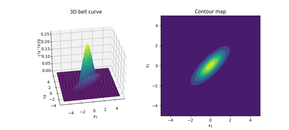
When the number of dimensions in $\mathbf{X}$, $D=2$, this special case of MVN is referred as Bivariate Normal (BVN).

An example of an BVN, $\mathcal{N}\left(\left[\begin{smallmatrix}0\\0\end{smallmatrix}\right],\left[\begin{smallmatrix}1&0.5\\0.8&1\end{smallmatrix}\right]\right)$, is shown as following.

Properties of the Covariance Matrix

Symmetric

With the definition \eqref{eq:mvn.1} of the covariance matrix $\boldsymbol{\Sigma}$, we can easily see that it is symmetric. However, notice that in the illustration of BVN, we gave the distribution a non-symmetric covariance matrix. The reason why we could do that is without loss of generality, we can assume that $\boldsymbol{\Sigma}$ is symmetric.

To prove this property, first off consider a square matrix $\mathbf{S}$, we have it can be written by \begin{equation} \mathbf{S}=\frac{\mathbf{S}+\mathbf{S}^\text{T}}{2}+\frac{\mathbf{S}-\mathbf{S}^\text{T}}{2}=\mathbf{S}_\text{S}+\mathbf{S}_\text{A}, \end{equation} where \begin{equation} \mathbf{S}_\text{S}=\frac{\mathbf{S}+\mathbf{S}^\text{T}}{2},\hspace{2cm}\mathbf{S}_\text{A}=\frac{\mathbf{S}-\mathbf{S}^\text{T}}{2} \end{equation} It is easily seen that $\mathbf{S}_\text{S}$ is symmetric because the $\{i,j\}$ element of its equal to the $\{j,i\}$ element due to \begin{equation} (\mathbf{S}_\text{S})_{ij}=\frac{(\mathbf{S})_{ij}+(\mathbf{S}^\text{T})_{ij}}{2}=\frac{(\mathbf{S}^\text{T})_{ji}+(\mathbf{S})_{ji}}{2}=(\mathbf{S}_\text{S})_{ji} \end{equation} On the other hand, the matrix $\mathbf{S}_\text{A}$ is anti-symmetric since \begin{equation} (\mathbf{S}_\text{A})_{ij}=\frac{(\mathbf{S})_{ij}-(\mathbf{S}^\text{T})_{ij}}{2}=\frac{(\mathbf{S}^\text{T})_{ji}-(\mathbf{S})_{ji}}{2}=-(\mathbf{S}_\text{A})_{ji} \end{equation} Consider the density of a distribution $\mathcal{N}(\boldsymbol{\mu},\boldsymbol{\Sigma})$, we have that $\boldsymbol{\Sigma}$ is square and so is its inverse $\boldsymbol{\Sigma}^{-1}$. Therefore we can express $\boldsymbol{\Sigma}^{-1}$ as a sum of a symmetric matrix $\boldsymbol{\Sigma}_\text{S}$ with an anti-symmetric matrix $\boldsymbol{\Sigma}_\text{A}$ \begin{equation} \boldsymbol{\Sigma}^{-1}=\boldsymbol{\Sigma}_\text{S}+\boldsymbol{\Sigma}_\text{A} \end{equation} We have that the density of the distribution is given by \begin{align} f(\mathbf{x})&=\frac{1}{(2\pi)^{D/2}\vert\boldsymbol{\Sigma}\vert^{1/2}}\exp\left[-\dfrac{1}{2}\left(\mathbf{x}-\boldsymbol{\mu}\right)^\text{T}\mathbf{\Sigma}^{-1}(\mathbf{x}-\boldsymbol{\mu})\right] \\ &\propto\exp\left[-\dfrac{1}{2}\left(\mathbf{x}-\boldsymbol{\mu}\right)^\text{T}\mathbf{\Sigma}^{-1}(\mathbf{x}-\boldsymbol{\mu})\right] \\ &=\exp\left[-\dfrac{1}{2}\left(\mathbf{x}-\boldsymbol{\mu}\right)^\text{T}(\boldsymbol{\Sigma}_\text{S}+\boldsymbol{\Sigma}_\text{A})(\mathbf{x}-\boldsymbol{\mu})\right] \\ &\propto\exp\left[\mathbf{v}^\text{T}\boldsymbol{\Sigma}_\text{S}\mathbf{v}+\mathbf{v}^\text{T}\boldsymbol{\Sigma}_\text{A}\mathbf{v}\right] \\ &=\exp\left[\mathbf{v}^\text{T}\boldsymbol{\Sigma}_\text{S}\mathbf{v}\right] \end{align} where in the forth step, we have defined $\mathbf{v}\doteq\mathbf{x}-\boldsymbol{\mu}$, and where in the fifth-step, the result obtained was due to \begin{align} \mathbf{v}^\text{T}\boldsymbol{\Sigma}_\text{A}\mathbf{v}&=\sum_{i=1}^{D}\sum_{j=1}^{D}\mathbf{v}_i(\boldsymbol{\Sigma}_\text{A})_{ij}\mathbf{v}_j \\ &=\sum_{i=1}^{D}\sum_{j=1}^{D}\mathbf{v}_i-(\boldsymbol{\Sigma}_\text{A})_{ji}\mathbf{v}_j \\ &=-\mathbf{v}^\text{T}\boldsymbol{\Sigma}_\text{A}\mathbf{v} \end{align} which implies that $\mathbf{v}^\text{T}\boldsymbol{\Sigma}_\text{A}\mathbf{v}=0$.

Thus, when computing the density, the symmetric part of $\boldsymbol{\Sigma}^{-1}$ is the only one matters. Or in other words, without loss of generality, we can assume that $\boldsymbol{\Sigma}^{-1}$ is symmetric, which means that $\boldsymbol{\Sigma}$ is also symmetric.

With this assumption of symmetry, the covariance matrix $\boldsymbol{\Sigma}$ now has all the properties of a symmetric matrix, as following in the next two sections.

Real eigenvalues

Consider an eigenvector, eigenvalue pair $(\mathbf{v},\lambda)$ of covariance matrix $\boldsymbol{\Sigma}$, we have \begin{equation} \boldsymbol{\Sigma}\mathbf{v}=\lambda\mathbf{v}\label{eq:rc.1} \end{equation} Since $\boldsymbol{\Sigma}\in\mathbb{R}^{D\times D}$, we have $\boldsymbol{\Sigma}=\overline{\boldsymbol{\Sigma}}$. Conjugate both sides of the equation above we have \begin{equation} \boldsymbol{\Sigma}\overline{\mathbf{v}}=\overline{\lambda}\overline{\mathbf{v}},\label{eq:rc.2} \end{equation} Since $\boldsymbol{\Sigma}$ is symmetric, we have $\boldsymbol{\Sigma}=\boldsymbol{\Sigma}^\text{T}$. Taking the transpose of both sides of \eqref{eq:rc.2} gives us \begin{equation} \overline{\mathbf{v}}^\text{T}\boldsymbol{\Sigma}=\overline{\lambda}\overline{\mathbf{v}}^\text{T}\label{eq:rc.3} \end{equation} Continuing by taking dot product of both sides of \eqref{eq:rc.3} with $\mathbf{v}$ lets us obtain \begin{equation} \overline{\mathbf{v}}^\text{T}\boldsymbol{\Sigma}\mathbf{v}=\overline{\lambda}\overline{\mathbf{v}}^\text{T}\mathbf{v}\label{eq:rc.4} \end{equation} On the other hand, take dot product of $\overline{\mathbf{v}}^\text{T}$ with both sides of \eqref{eq:rc.1}, we have \begin{equation} \overline{\mathbf{v}}^\text{T}\boldsymbol{\Sigma}\mathbf{v}=\lambda\overline{\mathbf{v}}^\text{T}\mathbf{v} \end{equation} which by \eqref{eq:rc.4} implies that \begin{equation} \overline{\lambda}\overline{\mathbf{v}}^\text{T}\mathbf{v}=\lambda\overline{\mathbf{v}}^\text{T}\mathbf{v}, \end{equation} or \begin{equation} (\lambda-\overline{\lambda})\overline{\mathbf{v}}^\text{T}\mathbf{v}=0\label{eq:rc.5} \end{equation} Moreover, we have that \begin{equation} \overline{\mathbf{v}}^\text{T}\mathbf{v}=\sum_{k=1}^{D}(a_k-i b_k)(a_k+i b_k)=\sum_{k=1}^{D}a^2+b^2>0 \end{equation} where we have denoted the complex eigenvector $\mathbf{v}\neq\mathbf{0}$ as \begin{equation} \mathbf{v}=(a_1+i b_1,\ldots,a_D+i b_D)^\text{T}, \end{equation} which implies that its complex conjugate $\overline{\mathbf{v}}$ can be written by \begin{equation} \overline{\mathbf{v}}=(a_1-i b_1,\ldots,a_D-i b_D)^\text{T} \end{equation} Therefore, by \eqref{eq:rc.5}, we can claim that \begin{equation} \lambda=\overline{\lambda} \end{equation} or in other words, the eigenvalue $\lambda$ of $\boldsymbol{\Sigma}$ is real.

Projection onto eigenvectors

First, we have that eigenvectors $\mathbf{v}_i$ and $\mathbf{v}_j$ corresponding to different eigenvalues $\lambda_i$ and $\lambda_j$ of $\boldsymbol{\Sigma}$ are perpendicular, because \begin{align} \lambda_i\mathbf{v}_i^\text{T}\mathbf{v}_j&=\mathbf{v}_i^\text{T}\boldsymbol{\Sigma}^\text{T}\mathbf{v}_j \\ &=\mathbf{v}_i^\text{T}\boldsymbol{\Sigma}\mathbf{v}_j=\mathbf{v}_i^\text{T}\lambda_j\mathbf{v}_j, \end{align} which implies that \begin{equation} (\lambda_i-\lambda_j)\mathbf{v}_i^\text{T}\mathbf{v}_j=0 \end{equation} Therefore, $\mathbf{v}_i^\text{T}\mathbf{v}_j=0$ since $\lambda_i\neq\lambda_j$.

Hence, for any unit eigenvectors $\mathbf{q}_i,\mathbf{q}_j$ of $\boldsymbol{\Sigma}$, we have \begin{equation} \mathbf{q}_i^\text{T}\mathbf{q}_j\begin{cases}1,&\hspace{0.5cm}\text{if }i=j \\ 0,&\hspace{0.5cm}\text{if }i\neq j\end{cases} \end{equation} This allows us to write $\boldsymbol{\Sigma}$ as \begin{equation} \boldsymbol{\Sigma}=\mathbf{Q}^\text{T}\boldsymbol{\Lambda}\mathbf{Q}, \end{equation} where $\mathbf{Q}$ is the orthonormal matrix whose $i$-th row is $\mathbf{q}_i^\text{T}$ and $\boldsymbol{\Lambda}$ is the diagonal matrix whose $\{i,i\}$ element is $\lambda_i$, as \begin{equation} \mathbf{Q}=\left[\begin{matrix}-\hspace{0.15cm}\mathbf{q}_1^\text{T}\hspace{0.15cm}- \\ \vdots \\ -\hspace{0.15cm}\mathbf{q}_D^\text{T}\hspace{0.15cm}-\end{matrix}\right],\hspace{2cm}\boldsymbol{\Lambda}=\left[\begin{matrix}\lambda_1&& \\ &\ddots& \\ &&\lambda_D\end{matrix}\right] \end{equation} Therefore, we can also write $\boldsymbol{\Sigma}$ as \begin{equation} \boldsymbol{\Sigma}=\sum_{i=1}^{D}\lambda_i\mathbf{q}_i\mathbf{q}_i^\text{T} \end{equation} Each matrix $\mathbf{q}_i\mathbf{q}_i^\text{T}$ is the projection matrix onto $\mathbf{q}_i$, then $\boldsymbol{\Sigma}$ can be express as a combination of perpendicular projection matrices.

Other than that, for any eigenvector, eigenvalue pair $(\mathbf{q_i},\lambda_i)$ of the matrix $\boldsymbol{\Sigma}$, we have \begin{align} \lambda_i\boldsymbol{\Sigma}^{-1}\mathbf{q}_i=\boldsymbol{\Sigma}^{-1}\boldsymbol{\Sigma}\mathbf{q}_i=\mathbf{q}_i \end{align} or \begin{equation} \boldsymbol{\Sigma}^{-1}\mathbf{q}_i=\frac{1}{\lambda_i}\mathbf{q}_i, \end{equation} which implies that each eigenvector, eigenvalue pair $(\mathbf{q_i},\lambda_i)$ of $\boldsymbol{\Sigma}$ corresponds to an eigenvector, eigenvalue pair $(\mathbf{q}_i,1/\lambda_i)$ of $\boldsymbol{\Sigma}^{-1}$. Therefore, $\boldsymbol{\Sigma}^{-1}$ can also be written by \begin{equation} \boldsymbol{\Sigma}^{-1}=\sum_{i=1}^{D}\frac{1}{\lambda_i}\mathbf{q}_i\mathbf{q}_i^\text{T}\label{eq:pec.1} \end{equation}

Properties of Normal Distribution

An crucial property of the multivariate Normal distribution is that if two sets of variables are jointly Gaussian, then the conditional probability distribution of one set given the other is then also Gaussian. Analogously, the marginal of either set is Gaussian too.

Conditional Gaussian Distribution

Let $\mathbf{x}$ be a $D$-dimensional random vector such that $\mathbf{x}\sim\mathcal{N}(\boldsymbol{\mu},\boldsymbol{\Sigma})$, and that we partition $\mathbf{x}$ into two disjoint subsets $\mathbf{x}_a$ and $\mathbf{x}_b$ with $\mathbf{x}_a$ is an $M$-dimensional vector and $\mathbf{x}_b$ is a $(D-M)$-dimensional vector. \begin{equation} \mathbf{x}=\left[\begin{matrix}\mathbf{x}_a \\ \mathbf{x}_b\end{matrix}\right] \end{equation} Along with them, we also define their corresponding means, as a partition of $\boldsymbol{\mu}$ \begin{equation} \boldsymbol{\mu}=\left[\begin{matrix}\boldsymbol{\mu}_a \\ \boldsymbol{\mu}_b\end{matrix}\right] \end{equation} and their corresponding covariance matrices \begin{equation} \boldsymbol{\Sigma}=\left[\begin{matrix}\boldsymbol{\Sigma}_{aa}&\boldsymbol{\Sigma}_{ab} \\ \boldsymbol{\Sigma}_{b a}&\boldsymbol{\Sigma}_{bb}\end{matrix}\right], \end{equation} which implies that $\boldsymbol{\Sigma}_{ab}=\boldsymbol{\Sigma}_{b a}^\text{T}$.

Analogously, we also define the partitioned form of the precision matrix $\boldsymbol{\Sigma}^{-1}$ \begin{equation} \boldsymbol{\Lambda}\doteq\boldsymbol{\Sigma}^{-1}=\left[\begin{matrix}\boldsymbol{\Lambda}_{aa}&\boldsymbol{\Lambda}_{ab} \\ \boldsymbol{\Lambda}_{ba}&\boldsymbol{\Lambda}_{bb}\end{matrix}\right], \end{equation} Thus, we also have that $\boldsymbol{\Lambda}_{ab}=\boldsymbol{\Lambda}_{ba}^\text{T}$ since $\boldsymbol{\Sigma}^{-1}$ or in other words, $\boldsymbol{\Lambda}$ is symmetric due to the symmetry of $\boldsymbol{\Sigma}$. With these partitions, we can rewrite the functional dependence of the Gaussian \eqref{eq:mvn.2} on $\mathbf{x}$ as \begin{align} \hspace{-1.2cm}-\frac{1}{2}(\mathbf{x}-\boldsymbol{\mu})^\text{T}\boldsymbol{\Sigma}^{-1}(\mathbf{x}-\boldsymbol{\mu})&=-\frac{1}{2}(\mathbf{x}_a-\boldsymbol{\mu}_a)^\text{T}\boldsymbol{\Lambda}_{aa}(\mathbf{x}_a-\boldsymbol{\mu}_a)-\frac{1}{2}(\mathbf{x}_a-\boldsymbol{\mu}_a)^\text{T}\boldsymbol{\Lambda}_{ab}(\mathbf{x}_b-\boldsymbol{\mu}_b) \\ &\hspace{0.5cm}-\frac{1}{2}(\mathbf{x}_b-\boldsymbol{\mu}_b)^\text{T}\boldsymbol{\Lambda}_{ba}(\mathbf{x}_a-\boldsymbol{\mu}_a)-\frac{1}{2}(\mathbf{x}_b-\boldsymbol{\mu}_b)^\text{T}\boldsymbol{\Lambda}_{bb}(\mathbf{x}_b-\boldsymbol{\mu}_b)\label{eq:cgd.1} \end{align} Consider the conditional probability $p(\mathbf{x}_a\vert\mathbf{x}_b)$, which is the distribution of $\mathbf{x}_a$ given $\mathbf{x}_b$. Viewing $\mathbf{x}_b$ as a constant, \eqref{eq:cgd.1} will be the functional dependence of the conditional probability $p(\mathbf{x}_a\vert\mathbf{x}_b)$ on $\mathbf{x}_a$, which can be continued to derive as \begin{align} &-\frac{1}{2}\mathbf{x}_a^\text{T}\boldsymbol{\Lambda}_{aa}\mathbf{x}_a+\frac{1}{2}\mathbf{x}_a^\text{T}\big(\boldsymbol{\Lambda}_{aa}\boldsymbol{\mu}_a+\boldsymbol{\Lambda}_{aa}^\text{T}\boldsymbol{\mu}_a-\boldsymbol{\Lambda}_{ab}\mathbf{x}_b+\boldsymbol{\Lambda}_{ab}\boldsymbol{\mu}_b-\boldsymbol{\Lambda}_{ba}^\text{T}\mathbf{x}_b+\boldsymbol{\Lambda}_{ba}\boldsymbol{\mu}_b\big)+c \\ &\hspace{3cm}=-\frac{1}{2}\mathbf{x}_a^\text{T}\boldsymbol{\Lambda}_{aa}\mathbf{x}_a+\mathbf{x}_a^\text{T}\big(\boldsymbol{\Lambda}_{aa}\boldsymbol{\mu}_a-\boldsymbol{\Lambda}_{ab}(\mathbf{x}_b-\boldsymbol{\mu}_b)\big)+c,\label{eq:cgd.2} \end{align} where $c$ is a constant, and we have used the $\boldsymbol{\Lambda}_{aa}=\boldsymbol{\Lambda}_{aa}^\text{T}$ and $\boldsymbol{\Lambda}_{ab}=\boldsymbol{\Lambda}_{ba}^\text{T}$.

Moreover, we have that the variation part which depends on $\mathbf{x}$ for any Gaussian $\mathbf{X}\sim\mathcal{N}(\mathbf{x}\vert\boldsymbol{\mu},\boldsymbol{\Sigma})$ can be written as a quadratic function of $\mathbf{x}$ \begin{equation} -\frac{1}{2}(\mathbf{x}-\boldsymbol{\mu})^\text{T}\boldsymbol{\Sigma}^{-1}(\mathbf{x}-\boldsymbol{\mu})=-\frac{1}{2}\mathbf{x}^\text{T}\boldsymbol{\Sigma}^{-1}\mathbf{x}+\mathbf{x}^\text{T}\boldsymbol{\Sigma}^{-1}\boldsymbol{\mu}+c,\label{eq:cgd.3} \end{equation} where $c$ is a constant. With this observation, and by \eqref{eq:cgd.2} we have that the conditional distribution $p(\mathbf{x}_a\vert\mathbf{x}_b)$ is a Gaussian, with the corresponding covariance matrix, denoted as $\boldsymbol{\Sigma}_{a\vert b}$, given by \begin{equation} \boldsymbol{\Sigma}_{a\vert b}=\boldsymbol{\Lambda}_{aa}^{-1},\label{eq:cgd.4} \end{equation} and with the corresponding mean vector, denoted as $\boldsymbol{\mu}_{a\vert b}$, given by \begin{align} \boldsymbol{\mu}_{a\vert b}&=\boldsymbol{\Sigma}_{a\vert b}\big(\boldsymbol{\Lambda}_{aa}\boldsymbol{\mu}_a-\boldsymbol{\Lambda}_{ab}(\mathbf{x}_b-\boldsymbol{\mu}_b)\big) \\ &=\boldsymbol{\mu}_a-\boldsymbol{\Lambda}_{aa}^{-1}\boldsymbol{\Lambda}_{ab}(\mathbf{x}_b-\boldsymbol{\mu}_b)\label{eq:cgd.5} \end{align} To express the mean $\boldsymbol{\mu}_{a\vert b}$ and the covariance matrix $\boldsymbol{\Sigma}_{a\vert b}$ of $p(\mathbf{x}_a\vert\mathbf{x}_b)$ in terms of partition of the covariance matrix $\boldsymbol{\Sigma}$ instead of the precision matrix $\boldsymbol{\Lambda}$’s, we will be using the identity for the inverse of a partitioned matrix \begin{align} \left[\begin{matrix}\mathbf{A}&\mathbf{B} \\ \mathbf{C}&\mathbf{D}\end{matrix}\right]^{-1}=\left[\begin{matrix}\mathbf{M}&-\mathbf{M}\mathbf{B}\mathbf{D}^{-1} \\ -\mathbf{D}^{-1}\mathbf{C}\mathbf{M}&\mathbf{D}^{-1}+\mathbf{D}^{-1}\mathbf{C}\mathbf{M}\mathbf{B}\mathbf{D}^{-1}\end{matrix}\right],\label{eq:cgd.6} \end{align} where we have defined \begin{equation} \mathbf{M}\doteq(\mathbf{A}-\mathbf{B}\mathbf{D}^{-1}\mathbf{C})^{-1}, \end{equation} whose inverse $\mathbf{M}^{-1}$ is called the Schur complement of the matrix $\left[\begin{matrix}\mathbf{A}&\mathbf{B} \\ \mathbf{C}&\mathbf{D}\end{matrix}\right]^{-1}$. This identity can be proved by multiplying both sides of \eqref{eq:cgd.6} with $\left[\begin{matrix}\mathbf{A}&\mathbf{B} \\ \mathbf{C}&\mathbf{D}\end{matrix}\right]$ to give \begin{align} \mathbf{I}&=\left[\begin{matrix}\mathbf{M}&-\mathbf{M}\mathbf{B}\mathbf{D}^{-1} \\ -\mathbf{D}^{-1}\mathbf{C}\mathbf{M}&\mathbf{D}^{-1}+\mathbf{D}^{-1}\mathbf{C}\mathbf{M}\mathbf{B}\mathbf{D}^{-1}\end{matrix}\right]\left[\begin{matrix}\mathbf{A}&\mathbf{B} \\ \mathbf{C}&\mathbf{D}\end{matrix}\right] \\ &=\left[\begin{matrix}\mathbf{M}(\mathbf{A}-\mathbf{B}\mathbf{D}^{-1}\mathbf{C})&\mathbf{M}\mathbf{B}-\mathbf{M}\mathbf{B} \\ -\mathbf{D}^{-1}\mathbf{C}\mathbf{M}\mathbf{A}+\mathbf{D}^{-1}\mathbf{C}+\mathbf{D}^{-1}\mathbf{C}\mathbf{M}\mathbf{B}\mathbf{D}^{-1}\mathbf{C}&-\mathbf{D}^{-1}\mathbf{C}\mathbf{M}\mathbf{B}+\mathbf{I}+\mathbf{D}^{-1}\mathbf{C}\mathbf{M}\mathbf{B}\end{matrix}\right] \\ &=\left[\begin{matrix}\mathbf{I}&\mathbf{0} \\ \mathbf{D}^{-1}\mathbf{C}\big(\mathbf{I}-\mathbf{M}(\mathbf{A}-\mathbf{B}\mathbf{D}^{-1}\mathbf{C})\big)&\mathbf{I}\end{matrix}\right] \\ &=\left[\begin{matrix}\mathbf{I}&\mathbf{0} \\ \mathbf{0}&\mathbf{I}\end{matrix}\right]=\mathbf{I}, \end{align} which claims our argument.

Applying the identity \eqref{eq:cgd.6} into the precision matrix $\boldsymbol{\Lambda}=\boldsymbol{\Sigma}^{-1}$ gives us \begin{equation} \hspace{-0.5cm}\left[\begin{matrix}\boldsymbol{\Lambda}_{aa}&\boldsymbol{\Lambda}_{ab} \\ \boldsymbol{\Lambda}_{ba}&\boldsymbol{\Lambda}_{bb}\end{matrix}\right]=\left[\begin{matrix}\boldsymbol{\Sigma}_{aa}&\boldsymbol{\Sigma}_{ab} \\ \boldsymbol{\Sigma}_{b a}&\boldsymbol{\Sigma}_{bb}\end{matrix}\right]^{-1}=\left[\begin{matrix}\mathbf{M}_\boldsymbol{\Sigma}&-\mathbf{M}_\boldsymbol{\Sigma}\boldsymbol{\Sigma}_{ab}\boldsymbol{\Sigma}_{bb}^{-1} \\ -\boldsymbol{\Sigma}_{bb}^{-1}\boldsymbol{\Sigma}_{ba}\mathbf{M}_\boldsymbol{\Sigma}&\boldsymbol{\Sigma}_{bb}^{-1}+\boldsymbol{\Sigma}_{bb}^{-1}\boldsymbol{\Sigma}_{ba}\mathbf{M}_\boldsymbol{\Sigma}\boldsymbol{\Sigma}_{ab}\boldsymbol{\Sigma}_{bb}^{-1}\end{matrix}\right], \end{equation} where the Schur complement of $\mathbf{\Sigma}^{-1}$ is given by \begin{equation} \mathbf{M}_\boldsymbol{\Sigma}=\big(\boldsymbol{\Sigma}_{aa}-\boldsymbol{\Sigma}_{ab}\boldsymbol{\Sigma}_{bb}^{-1}\boldsymbol{\Sigma}_{ba}\big)^{-1} \end{equation} Hence, we obtain \begin{align} \boldsymbol{\Lambda}_{aa}&=\mathbf{M}_\boldsymbol{\Sigma}=\big(\boldsymbol{\Sigma}_{aa}-\boldsymbol{\Sigma}_{ab}\boldsymbol{\Sigma}_{bb}^{-1}\boldsymbol{\Sigma}_{ba}\big)^{-1}, \\ \boldsymbol{\Lambda}_{ab}&=-\mathbf{M}_\boldsymbol{\Sigma}\boldsymbol{\Sigma}_{ab}\boldsymbol{\Sigma}_{bb}^{-1}=\big(\boldsymbol{\Sigma}_{aa}-\boldsymbol{\Sigma}_{ab}\boldsymbol{\Sigma}_{bb}^{-1}\boldsymbol{\Sigma}_{ba}\big)^{-1}\boldsymbol{\Sigma}_{ab}\boldsymbol{\Sigma}_{bb}^{-1} \end{align} Substitute these results into \eqref{eq:cgd.4} and \eqref{eq:cgd.5}, we have the mean and the covariance matrix of the conditional Gaussian distribution $p(\mathbf{x}_a\vert\mathbf{x}_b)$ can be rewritten as \begin{align} \boldsymbol{\mu}_{a\vert b}&=\boldsymbol{\mu}_a+\boldsymbol{\Sigma}_{ab}\boldsymbol{\Sigma}_{bb}^{-1}(\mathbf{x}_b-\boldsymbol{\mu}_b), \\ \boldsymbol{\Sigma}_{a\vert b}&=\boldsymbol{\Sigma}_{aa}-\boldsymbol{\Sigma}_{ab}\boldsymbol{\Sigma}_{bb}^{-1}\boldsymbol{\Sigma}_{ba} \end{align} It is worth noticing that the mean $\boldsymbol{\mu}_{a\vert b}$ given above is a linear function of $\mathbf{x}_b$, while the covariance matrix $\boldsymbol{\Sigma}_{a\vert b}$ is independent of $\mathbf{x}_b$. This is an example of a linear Gaussian model.

Marginal Gaussian Distribution

Given the settings as in previous section, let us consider the marginal distribution of $\mathbf{x}_a$, which can be computed by marginalizing the joint distribution \begin{equation} p(\mathbf{x}_a)=\int p(\mathbf{x}_a,\mathbf{x}_b)d\mathbf{x}_b\label{eq:mgd.1} \end{equation} which is an integration over $\mathbf{x}_b$, and thus terms that does not depend on $\mathbf{x}_b$ can be removed out of the integral.

Hence, using the result \eqref{eq:cgd.1}, the terms that the depends on $\mathbf{x}_b$ is \begin{align} &-\frac{1}{2}\Big[\mathbf{x}_b^\text{T}\boldsymbol{\Lambda}_{bb}\mathbf{x}_b+\mathbf{x}_b^\text{T}(\boldsymbol{\Lambda}_{bb}\boldsymbol{\mu}_b+\boldsymbol{\Lambda}_{bb}^\text{T}\boldsymbol{\mu}_b-\boldsymbol{\Lambda}_{ba}\mathbf{x}_a+\boldsymbol{\Lambda}_{ba}\boldsymbol{\mu}_a-\boldsymbol{\Lambda}_{ab}^\text{T}\mathbf{x}_a+\boldsymbol{\Lambda}_{ab}\boldsymbol{\mu}_a)\Big] \\ &=-\frac{1}{2}(\mathbf{x}_b-\boldsymbol{\Lambda}_{bb}^{-1}\mathbf{m})^\text{T}\boldsymbol{\Lambda}_{bb}(\mathbf{x}_b-\boldsymbol{\Lambda}_{bb}^{-1}\mathbf{m})+\frac{1}{2}\mathbf{m}^ \text{T}\boldsymbol{\Lambda}_{bb}^{-1}\mathbf{m},\label{eq:mgd.2} \end{align} where we have defined \begin{equation} \mathbf{m}=\boldsymbol{\Lambda}_{bb}\boldsymbol{\mu}_b-\boldsymbol{\Lambda}_{ba}(\mathbf{x}_a-\boldsymbol{\mu}_a) \end{equation} The first term in \eqref{eq:mgd.2} involves $\mathbf{x}_b$, while the second one, $\frac{1}{2}\mathbf{m}^\text{T}\boldsymbol{\Lambda}_{bb}^{-1}\mathbf{m}$, does not, but it does depend on $\mathbf{x}_a$. Thus the integration over $\mathbf{x}_b$ required in \eqref{eq:mgd.1} will take the form \begin{equation} \int\exp\left[-\frac{1}{2}(\mathbf{x}_b-\boldsymbol{\Lambda}_{bb}^{-1}\mathbf{m})^\text{T}\boldsymbol{\Lambda}_{bb}(\mathbf{x}_b-\boldsymbol{\Lambda}_{bb}^{-1}\mathbf{m})\right]d\mathbf{x}_b, \end{equation} which can be seen as an integral over an unnormalized Gaussian, and so the result will be the reciprocal of the normalizing coefficient. Moreover, from \eqref{eq:mvn.2}, we have that this coefficient is independent of the mean, $\boldsymbol{\Lambda}_{bb}^{-1}\mathbf{m}$, which involves $\mathbf{x}_a$, and depends only on the determinant of the covariance matrix, $\boldsymbol{\Lambda}_{bb}$, which does not involve $\mathbf{x}_a$. Therefore, using the result \eqref{eq:cgd.1} to select out the terms uninvolved $\mathbf{x}_b$, we have that \begin{align} &\frac{1}{2}\mathbf{m}^\text{T}\boldsymbol{\Lambda}_{bb}^{-1}\mathbf{m}-\frac{1}{2}\mathbf{x}_a^\text{T}\boldsymbol{\Lambda}_{aa}\mathbf{x}_a+\frac{1}{2}\mathbf{x}_a^\text{T}(\boldsymbol{\Lambda}_{aa}\boldsymbol{\mu}_a+\boldsymbol{\Lambda}_{aa}^\text{T}\boldsymbol{\mu}_a+\boldsymbol{\Lambda}_{ab}\boldsymbol{\mu}_b+\boldsymbol{\Lambda}_{ba}\boldsymbol{\mu}_b)+c\nonumber \\ &=-\frac{1}{2}\mathbf{x}_a^\text{T}(\boldsymbol{\Lambda}_{aa}-\boldsymbol{\Lambda}_{ab}\boldsymbol{\Lambda}_{bb}^{-1}\boldsymbol{\Lambda}_{ba})\mathbf{x}_a+\mathbf{x}_a^\text{T}(\boldsymbol{\Lambda}_{aa}-\boldsymbol{\Lambda}_{ab}\boldsymbol{\Lambda}_{bb}^{-1}\boldsymbol{\Lambda}_{ba})^{-1}\boldsymbol{\mu}_a+c, \end{align} where $c$ denotes the term that is independent of $\mathbf{x}_a$. Hence, using \eqref{eq:cgd.3} once again, we have that the marginal of $\mathbf{x}_a$, $p(\mathbf{x}_a)$, is also a Gaussian, with the corresponding covariance matrix, denoted $\boldsymbol{\Sigma}_a$, given by \begin{equation} \boldsymbol{\Sigma}=(\boldsymbol{\Lambda}_{aa}-\boldsymbol{\Lambda}_{ab}\boldsymbol{\Lambda}_{bb}^{-1}\boldsymbol{\Lambda}_{ba})^{-1}=\boldsymbol{\Sigma}_{aa},\label{eq:mgd.3} \end{equation} where we have used \eqref{eq:cgd.6} as in the conditional distribution. The mean of $p(\mathbf{x}_a)$ is then given as \begin{equation} \boldsymbol{\Sigma}_a(\boldsymbol{\Lambda}_{aa}-\boldsymbol{\Lambda}_{ab}\boldsymbol{\Lambda}_{bb}^{-1}\boldsymbol{\Lambda}_{ba}) \boldsymbol{\mu}_a=\boldsymbol{\mu}_a\label{eq:mgd.4} \end{equation}

Remark:
Given a joint Gaussian distribution $\mathcal{N}(\mathbf{x}\vert\boldsymbol{\mu},\boldsymbol{\Sigma})$ with precision matrix $\boldsymbol{\Lambda}\equiv\boldsymbol{\Sigma}^{-1}$ and \begin{align} \mathbf{x}&=\left[\begin{matrix}\mathbf{x}_a \\ \mathbf{x}_b\end{matrix}\right],&&\boldsymbol{\mu}=\left[\begin{matrix}\boldsymbol{\mu}_a \\ \boldsymbol{\mu}_b\end{matrix}\right] \\ \boldsymbol{\Sigma}&=\left[\begin{matrix}\boldsymbol{\Sigma}_{aa}&\boldsymbol{\Sigma}_{ab} \\ \boldsymbol{\Sigma}_{ba}&\boldsymbol{\Sigma}_{bb}\end{matrix}\right],&&\boldsymbol{\Lambda}=\left[\begin{matrix}\boldsymbol{\Lambda}_{aa}&\boldsymbol{\Lambda}_{aa} \\ \boldsymbol{\Lambda}_{ba}&\boldsymbol{\Lambda}_{bb}\end{matrix}\right] \end{align} The resulting conditional distribution is a Gaussian \begin{align} p(\mathbf{x}_a\vert\mathbf{x}_b)&=\mathcal{N}(\mathbf{x}\vert\boldsymbol{\mu}_{a\vert b},\boldsymbol{\Sigma}_{a\vert b}) \\ \boldsymbol{\mu}_{a\vert b}&=\boldsymbol{\mu}_a-\boldsymbol{\Lambda}_{aa}^{-1}\boldsymbol{\Lambda}_{ab}(\mathbf{x}_b-\boldsymbol{\mu}_b) \\ \boldsymbol{\Sigma}_{a\vert b}&=\boldsymbol{\Lambda}_{aa}^{-1}=\boldsymbol{\Sigma}_{aa}-\boldsymbol{\Sigma}_{ab}\boldsymbol{\Sigma}_{bb}^{-1}\boldsymbol{\Sigma}_{ba} \end{align} Also, the marginal distribution is a Gaussian \begin{equation} p(\mathbf{x}_a)=\mathcal{N}(\mathbf{x}_a\vert\boldsymbol{\mu}_a,\boldsymbol{\Sigma}_{aa}) \end{equation}

Bayes’ theorem for Gaussian variables

In this section, we will apply the Bayes’ theorem to find the marginal distribution of $p(\mathbf{y})$ and conditional distribution $p(\mathbf{x}\vert\mathbf{y})$ with supposing that we are given a Gaussian distribution $p(\mathbf{x})$ and a conditional Gaussian distribution $p(\mathbf{y}\vert\mathbf{x})$ in which $p(\mathbf{y}\vert\mathbf{x})$ has a mean that is a linear function of $\mathbf{x}$, and a covariance matrix which is independent of $\mathbf{x}$, as \begin{align} p(\mathbf{x})&=\mathcal{N}(\mathbf{x}\vert\boldsymbol{\mu},\boldsymbol{\Lambda}^{-1}), \\ p(\mathbf{y}\vert\mathbf{x})&=\mathcal{N}(\mathbf{y}\vert\mathbf{A}\mathbf{x}+\mathbf{b},\mathbf{L}^{-1}), \end{align} where $\mathbf{A},\mathbf{b}$ are two parameters controlling the means, and $\boldsymbol{\Lambda},\boldsymbol{L}$ are precision matrices.

In order to find the marginal and conditional distribution, first we will be looking for the joint distribution $p(\mathbf{x},\mathbf{y})$ by considering the augmented vector \begin{equation} \mathbf{z}=\left[\begin{matrix}\mathbf{x} \\ \mathbf{y}\end{matrix}\right] \end{equation} Therefore, we have \begin{equation} p(\mathbf{z})=p(\mathbf{x},\mathbf{y})=p(\mathbf{x})p(\mathbf{y}\vert\mathbf{x}) \end{equation} Taking the natural logarithm of both sides gives us \begin{align} \log p(\mathbf{z})&=\log p(\mathbf{x})+\log p(\mathbf{y}\vert\mathbf{x}) \\ &=\log\mathcal{N}(\mathbf{x}\vert\boldsymbol{\mu},\boldsymbol{\Lambda}^{-1})+\log\mathcal{N}(\mathbf{y}\vert\mathbf{A}\mathbf{x}+\mathbf{b},\mathbf{L}^{-1}) \\ &=-\frac{1}{2}(\mathbf{x}-\boldsymbol{\mu})^\text{T}\boldsymbol{\Lambda}(\mathbf{x}-\boldsymbol{\mu})-\frac{1}{2}(\mathbf{y}-\mathbf{A}\mathbf{x}-\mathbf{b})^\text{T}\mathbf{L}(\mathbf{y}-\mathbf{A}\mathbf{x}-\mathbf{b})+c\label{eq:btg.1} \end{align} where $c$ is a constant in terms of $\mathbf{x}$ and $\mathbf{y}$, i.e., $c$ is independent of $\mathbf{x},\mathbf{y}$.

It is easily to notice that \eqref{eq:btg.1} is a quadratic function of the components of $\mathbf{z}$, which implies that $p(\mathbf{z})$ is a Gaussian. By \eqref{eq:cgd.3}, in order to find the covariance matrix of $\mathbf{z}$, we consider the quadratic terms in \eqref{eq:btg.1}, which are given by \begin{align} &-\frac{1}{2}\mathbf{x}^\text{T}\boldsymbol{\Lambda}\mathbf{x}-\frac{1}{2}(\mathbf{y}-\mathbf{A}\mathbf{x})^\text{T}\mathbf{L}(\mathbf{y}-\mathbf{A}\mathbf{x}) \\ &=-\frac{1}{2}\Big[\mathbf{x}^\text{T}\big(\boldsymbol{\Lambda}+\mathbf{A}^\text{T}\mathbf{L}\mathbf{A}\big)\mathbf{x}+\mathbf{y}^\text{T}\mathbf{L}\mathbf{y}-\mathbf{y}^\text{T}\mathbf{L}\mathbf{A}\mathbf{x}-\mathbf{x}^\text{T}\mathbf{A}^\text{T}\mathbf{L}\mathbf{y}\Big] \\ &=-\frac{1}{2}\left[\begin{matrix}\mathbf{x} \\ \mathbf{y}\end{matrix}\right]^\text{T}\left[\begin{matrix}\boldsymbol{\Lambda}+\mathbf{A}^\text{T}\mathbf{L}\mathbf{A}&-\mathbf{A}^\text{T}\mathbf{L} \\ -\mathbf{L}\mathbf{A}&\mathbf{L}\end{matrix}\right]\left[\begin{matrix}\mathbf{x} \\ \mathbf{y}\end{matrix}\right] \\ &=-\frac{1}{2}\mathbf{z}^\text{T}\mathbf{R}\mathbf{z}, \end{align} which implies that the precision matrix of $\mathbf{z}$ is $\mathbf{R}$, defined as \begin{equation} \mathbf{R}=\left[\begin{matrix}\boldsymbol{\Lambda}+\mathbf{A}^\text{T}\mathbf{L}\mathbf{A}&-\mathbf{A}^\text{T}\mathbf{L} \\ -\mathbf{L}\mathbf{A}&\mathbf{L}\end{matrix}\right] \end{equation} Thus, using the identity \eqref{eq:cgd.6}, we obtain the covariance matrix of the joint distribution \begin{equation} \boldsymbol{\Sigma}_\mathbf{z}=\mathbf{R}^{-1}=\left[\begin{matrix}\boldsymbol{\Lambda}^{-1}&\boldsymbol{\Lambda}^{-1}\mathbf{A}^\text{T} \\ \mathbf{A}\boldsymbol{\Lambda}^{-1}&\mathbf{L}^{-1}+\mathbf{A}\boldsymbol{\Lambda}^{-1}\mathbf{A}^\text{T}\end{matrix}\right] \end{equation} Analogously, by \eqref{eq:cgd.3}, we can find the mean of the joint distribution by considering the linear terms of \eqref{eq:btg.1}, which are \begin{align} \hspace{-0.7cm}\frac{1}{2}\Big[\mathbf{x}^\text{T}\boldsymbol{\Lambda}\boldsymbol{\mu}+\boldsymbol{\mu}^\text{T}\boldsymbol{\Lambda}\mathbf{x}+(\mathbf{y}-\mathbf{A}\mathbf{x})^\text{T}\mathbf{L}\mathbf{b}+\mathbf{b}^\text{T}\mathbf{L}(\mathbf{y}-\mathbf{A}\mathbf{x}) \Big]&=\mathbf{x}^\text{T}\boldsymbol{\Lambda}\boldsymbol{\mu}-\mathbf{x}^\text{T}\mathbf{A}^\text{T}\mathbf{L}\mathbf{b}+\mathbf{y}^\text{T}\mathbf{L}\mathbf{b} \\ &=\left[\begin{matrix}\mathbf{x} \\ \mathbf{y}\end{matrix}\right]^\text{T}\left[\begin{matrix}\boldsymbol{\Lambda}\boldsymbol{\mu}-\mathbf{A}^\text{T}\mathbf{L}\mathbf{b} \\ \mathbf{L}\mathbf{b}\end{matrix}\right] \end{align} Thus, by \eqref{eq:cgd.3}, we have that the mean of the joint distribution is then given by \begin{equation} \boldsymbol{\mu}_\mathbf{z}=\boldsymbol{\Sigma}_\mathbf{z}\left[\begin{matrix}\boldsymbol{\Lambda}\boldsymbol{\mu}-\mathbf{A}^\text{T}\mathbf{L}\mathbf{b} \\ \mathbf{L}\mathbf{b}\end{matrix}\right]=\left[\begin{matrix}\boldsymbol{\mu} \\ \mathbf{A}\boldsymbol{\mu}+\mathbf{b}\end{matrix}\right] \end{equation} Given the mean $\boldsymbol{\mu}_\mathbf{z}$ and the covariance matrix $\boldsymbol{\Sigma}_\mathbf{z}$ of the joint distribution of $\mathbf{x},\mathbf{y}$, by \eqref{eq:mgd.3} and \eqref{eq:mgd.4}, we then can obtain the mean of the covariance matrix of the marginal distribution $p(\mathbf{y})$, which are \begin{align} \boldsymbol{\mu}_\mathbf{y}&=\mathbf{A}\boldsymbol{\mu}+\mathbf{b}, \\ \boldsymbol{\Sigma}_\mathbf{y}&=\mathbf{L}^{-1}+\mathbf{A}\boldsymbol{\Lambda}^{-1}\mathbf{A}^\text{T}, \end{align} and also, by \eqref{eq:cgd.4} and \eqref{eq:cgd.5}, we can easily get mean and covariance matrix of the conditional distribution $p(\mathbf{x}\vert\mathbf{y})$, which are given by \begin{align} \boldsymbol{\mu}_{\mathbf{x}\vert\mathbf{y}}&=(\boldsymbol{\Lambda}+\mathbf{A}^\text{T}\mathbf{L}\mathbf{A})^{-1}\big(\mathbf{A}^\text{T}\mathbf{L}(\mathbf{y}-\mathbf{b})+\boldsymbol{\Lambda}\boldsymbol{\mu}\big) \\ \boldsymbol{\Sigma}_{\mathbf{x}\vert\mathbf{y}}&=(\boldsymbol{\Lambda}+\mathbf{A}^\text{T}\mathbf{L}\mathbf{A})^{-1} \end{align} In Bayesian approach, we can consider $p(\mathbf{x})$ as a prior distribution over $\mathbf{x}$, and if $\mathbf{y}$ is observed, the conditional distribution $p(\mathbf{x}\vert\mathbf{y})$ will represents the corresponding posterior distribution over $\mathbf{x}$.

Remark:
Given a marginal Gaussian distribution for $\mathbf{x}$ and a conditional Gaussian distribution for $\mathbf{y}$ given $\mathbf{x}$ in the form \begin{align} p(\mathbf{x})&=\mathcal{N}(\mathbf{x}\vert\boldsymbol{\mu},\boldsymbol{\Lambda}^{-1}), \\ p(\mathbf{y}\vert\mathbf{x})&=\mathcal{N}(\mathbf{y}\vert\mathbf{A}\mathbf{x}+\mathbf{b},\mathbf{L}^{-1}), \end{align} the marginal distribution of $\mathbf{y}$ and the conditional distribution of $\mathbf{x}$ given $\mathbf{y}$ are then given by \begin{align} p(\mathbf{y})&=\mathcal{N}(\mathbf{y}\vert\mathbf{A}\boldsymbol{\mu}+\mathbf{b},\mathbf{L}^{-1}+\mathbf{A}\boldsymbol{\Lambda}^{-1}\mathbf{A}^\text{T}), \\ p(\mathbf{x}\vert\mathbf{y})&=\mathcal{N}(\mathbf{x}\vert\boldsymbol{\Sigma}(\mathbf{A}^\text{T}\mathbf{L}(\mathbf{y}-\mathbf{b})+\boldsymbol{\Lambda}\boldsymbol{\mu}),\boldsymbol{\Sigma}) \end{align} where \begin{equation} \boldsymbol{\Sigma}=(\boldsymbol{\Lambda}+\mathbf{A}^\text{T}\mathbf{L}\mathbf{A})^{-1} \end{equation}

Independencies in Normal Distributions

Theorem 1: Let $\mathbf{X}=X_1,\ldots,X_n$ have a joint Normal distribution $\mathcal{N}(\boldsymbol{\mu},\boldsymbol{\Sigma})$. Then $X_i$ and $X_j$ are independent iff $\boldsymbol{\Sigma}_{ij}=0$.

Proof
This can be easily proved by the formulas for conditional and marginal distributions obtained above and using the fact that \begin{equation} p\models X_i\perp X_j\Leftrightarrow p(X_i)=p(X_i\vert X_j) \end{equation}

Theorem 2: Consider a Gaussian distribution $p(X_1,\ldots,X_n)=\mathcal{N}(\boldsymbol{\mu},\boldsymbol{\Sigma})$, and let $\boldsymbol{\Lambda}=\boldsymbol{\Sigma}^{-1}$ denote the precision (information) matrix. Then \begin{equation} \boldsymbol{\Lambda}_{ij}=0\Leftrightarrow p\models(X_i\perp X_j\vert\mathcal{X}\backslash\{X_i,X_j\}) \end{equation}

Proof
Similarly, this can be proved by using the formula for conditional Gaussian, combined with the fact that \begin{equation} p\models(X_i\perp X_j\vert\mathcal{X}\backslash\{X_i,X_j\})\Leftrightarrow p(X_i\vert\mathcal{X}\backslash\{X_j\})=p(X_j\vert\mathcal{X}\backslash\{X_i\}) \end{equation}

Remark: It is followed by Theorem 2 that the information matrix $\boldsymbol{\Lambda}$ directly defines a minimal I-map Markov network for $p$. Specifically, by Theorem 15, since Gaussian is a positive distribution, we include an edge $X_i-X_j$ whenever $p\not\models(X_i\perp X_j\vert\mathcal{X}\backslash\{X_i,X_j\})$, which exactly when $\boldsymbol{\Lambda}_{ij}=0$.

Gaussian Bayesian Networks

We begin by first recalling the definition of linear Gaussian model: Let $Y$ be a continuous variable with continuous parents $X_1,\ldots,X_k$. We say that $Y$ has a linear Gaussian model if there are parameters $\beta_0,\ldots,\beta_k$ such that \begin{equation} p(Y\vert x_1,\ldots,x_k)=\mathcal{N}(\beta_0+\beta_1 x_1+\ldots+\beta_k x_k;\sigma^2), \end{equation} or \begin{equation} p(Y\vert\mathbf{x})=\mathcal{N}(\beta_0+\boldsymbol{\beta}^\text{T}\mathbf{x};\sigma^2) \end{equation} Thus, a Gaussian Bayesian network is a Bayesian network all of whose variables are continuous and where all of CPDs are linear Gaussian.

Theorem 3: Let $Y$ be a linear Gaussian of its parents $X_1,\ldots,X_k$, i.e. \begin{equation} p(Y\vert\mathbf{x})=\mathcal{N}(\beta_0+\boldsymbol{\beta}^\text{T}\mathbf{x};\sigma^2) \end{equation} Assume that $X_1,\ldots,X_k$ are jointly Gaussian with distribution $\mathcal{N}(\boldsymbol{\mu},\boldsymbol{\Sigma})$. Then

• The distribution of $Y$ is a Normal distribution $p(Y)=\mathcal{N}(\mu_Y;\sigma_Y^2)$ where \begin{align} \mu_Y&=\beta_0+\boldsymbol{\beta}^\text{T}\boldsymbol{\mu} \\ \sigma_Y^2&=\sigma^2+\boldsymbol{\beta}^\text{T}\boldsymbol{\Sigma}\boldsymbol{\beta} \end{align}
• The distribution over $\{\mathbf{X},Y\}$ is a Normal distribution where \begin{equation} \Cov(X_i,Y)=\sum_{j=1}^{k}\beta_j\boldsymbol{\Sigma}_{ij} \end{equation}

From this theorem, it follows by induction that if $\mathcal{B}$ is a linear Gaussian Bayesian network, then it defines a joint distribution that is jointly Gaussian.

The converse of this theorem is also true.

Theorem 4: Let $\{\mathbf{X},Y\}$ have a joint Normal distribution defined as usual \begin{equation} p(\mathbf{X},Y)=\mathcal{N}\left(\left[\begin{matrix}\boldsymbol{\mu}_\mathbf{X} \\ \boldsymbol{\mu}_Y\end{matrix}\right],\left[\begin{matrix}\boldsymbol{\Sigma}_{\mathbf{X}\mathbf{X}}&\boldsymbol{\Sigma}_{\mathbf{X}Y} \\ \boldsymbol{\Sigma}_{Y\mathbf{X}}&\boldsymbol{\Sigma}_{YY}\end{matrix}\right]\right) \end{equation} where since $Y\in\mathbb{R}$, we have that $\boldsymbol{\mu}_Y$ and $\boldsymbol{\Sigma}_{YY}$ are real numbers. Then the conditional distribution is a Gaussian \begin{equation} p(Y\vert\mathbf{X})=\mathcal{N}(\beta_0+\boldsymbol{\beta}^\text{T}\mathbf{X};\sigma^2), \end{equation} where \begin{align} \beta_0&=\boldsymbol{\mu}_Y-\boldsymbol{\Sigma}_{Y\mathbf{X}}\boldsymbol{\Sigma}_{\mathbf{X}\mathbf{X}}^{-1}\boldsymbol{\mu}_\mathbf{X} \\ \boldsymbol{\beta}&=\boldsymbol{\Sigma}_{\mathbf{X}\mathbf{X}}^{-1}\boldsymbol{\Sigma}_{Y\mathbf{X}} \\ \sigma^2&=\boldsymbol{\Sigma}_{YY}-\boldsymbol{\Sigma}_{Y\mathbf{X}}\boldsymbol{\Sigma}_{\mathbf{X}\mathbf{X}}^{-1}\boldsymbol{\Sigma}_{\mathbf{X}Y} \end{align} This theorem allows us to take a joint Gaussian distribution and produce a Bayesian network.

Theorem 5: Let $\mathcal{X}=\{X_1,\ldots,X_n\}$ be a set of r.v.s, and let $p$ be a joint Gaussian distribution over $\mathcal{X}$. Given any ordering $X_1,\ldots,X_n$ over $\mathcal{X}$, we can construct a Bayesian network structure $\mathcal{G}$ and a Bayesian network $\mathcal{B}$ over $\mathcal{G}$ such that

• $\text{Pa}_{X_i}^\mathcal{G}\subset\{X_1,\ldots,X_{i-1}\}$;
• the CPD of $X_i$ in $\mathcal{B}$ is a linear Gaussian of its parents;
• $\mathcal{G}$ is a minimal I-map for $p$.

References

[1] Joseph K. Blitzstein & Jessica Hwang. Introduction to Probability.

[2] Christopher M. Bishop. Pattern Recognition and Machine Learning. Springer New York, NY, 2006.

[3] Daphne Koller, Nir Friedman. Probabilistic Graphical Models. The MIT Press.

[4] Gilbert Strang. Introduction to Linear Algebra, 5th edition, 2016.

Footnotes