Read-through: Measure theory - Elementary measure, Jordan measure & the Riemann integral

Note I of the measure theory series. Materials are mostly taken from Tao’s book, except for some needed notations extracted from Stein’s book.

Preliminaries

Points, sets

A point $x\in\mathbb{R}^d$ consists of a $d$-tuple of real numbers \begin{equation} x=\left(x_1,x_2,\dots,x_d\right),\hspace{1cm}x_i\in\mathbb{R}, i=1,\dots,d \end{equation} Addition between points and multiplication of a point by a real scalar is elementwise.

The norm of $x$ is denoted by $\vert x\vert$ and is defined to be the standard Euclidean norm given by \begin{equation} \vert x\vert=\left(x_1^2+\dots+x_d^2\right)^{1/2} \end{equation} We can then calculate the distance between two points $x$ and $y$, which is \begin{equation} \text{dist}(x,y)=\vert x-y\vert \end{equation} The complement of a set $E$ in $\mathbb{R}^d$ is denoted as $E^c$, and defined by \begin{equation} E^c=\{x\in\mathbb{R}^d:x\notin E\} \end{equation} If $E$ and $F$ are two subsets of $\mathbb{R}^d$, we denote the complement of $F$ in $E$ by \begin{equation} E-F=\{x\in\mathbb{R}^d:x\in E;\hspace{0.1cm}x\notin F\} \end{equation} The distance between two sets $E$ and $F$ is defined by \begin{equation} \text{dist}(E,F)=\inf_{x\in E,\hspace{0.1cm}y\in F}\vert x-y\vert \end{equation}

Open, closed and compact sets

The open ball in $\mathbb{R}^d$ centered at $x$ and of radius $r$ is defined by \begin{equation} B(x,r)=\{y\in\mathbb{R}^d:\vert y-x\vert< r\} \end{equation} A subset $E\subset\mathbb{R}^d$ is open if for every $x\in E$ there exists $r>0$ with $B(x,r)\subset E$. And a set is closed if its complement is open.
Any (not necessarily countable) union of open sets is open, while in general, the intersection of only finitely many open sets is open. A similar statement holds for the class of closed sets, if we interchange the roles of unions and intersections.

A set $E$ is bounded if it is contained in some ball of finite radius. A set is compact if it is bounded and is also closed. Compact sets enjoy the Heine-Borel covering property:

Theorem 1. (Heine-Borel theorem)
Assume $E$ is compact, $E\subset\bigcup_\alpha\mathcal{O}_\alpha$, and each $\mathcal{O}_\alpha$ is open. Then there are finitely many of the open sets $\mathcal{O}_{\alpha_1},\mathcal{O}_{\alpha_2},\dots,\mathcal{O}_{\alpha_N}$, such that $E\subset\bigcup_{j=1}^{N}\mathcal{O}_{\alpha_j}$.

In words, any covering of a compact set by a collection of open sets contains a finite subcovering.

A point $x\in\mathbb{R}^d$ is a limit point of the set $E$ if for every $r>0$, the ball $B(x,r)$ contains points of $E$. This means that there are points in $E$ which are arbitrarily close to $x$. An isolated point of $E$ is a point $x\in E$ such that there exists an $r>0$ where $B(x,r)\cap E=\{x\}$.

A point $x\in E$ is an interior point of $E$ if there exists $r>0$ such that $B(x,r)\subset E$. The set of all interior points of $E$ is called the interior of $E$.

The closure of $E$, denoted as $\bar{E}$, consists the union of $E$ and all its limit points. The boundary of $E$, denoted as $\partial E$, is the set of points which are in the closure of $E$ but not in the interior of $E$.

A closed set $E$ is perfect if $E$ does not have any isolated point.

The boundary of $E$, denoted by $\partial E$, is the set of points in $\bar{E}$ not belonging to the interior of $E$.

Remark:

• The closure of a set is a closed set.
• Every point in $E$ is a limit point of $E$.
• A set is closed iff it contains all its limit points.

Rectangles, cubes

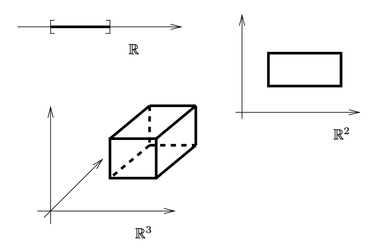
A (closed) rectangle $R$ in $\mathbb{R}^d$ is given by the product of $d$ one-dimensional closed and bounded intervals \begin{equation} R\doteq[a_1,b_1]\times[a_2,b_2]\times\ldots\times[a_d,b_d], \end{equation} where $a_j\leq b_j$, for $j=1,\ldots,d$, are real numbers. In other words, we have \begin{equation} R=\left\{\left(x_1,\ldots,x_d\right)\in\mathbb{R}^d:a_j\leq x_j\leq b_j,\forall j=1,\ldots,d\right\} \end{equation} With this definition, a rectangle is closed and has sides parallel to the coordinate axis. In $\mathbb{R}$, the rectangles are the closed and bounded intervals; they becomes the usual rectangles as we usually see in $\mathbb{R}^2$; while in $\mathbb{R}^3$, they are the closed parallelepipeds.

The lengths of the sides of the rectangle $R$ in $\mathbb{R}^d$ are $b_1-a_1,\ldots,b_d-a_d$. The volume of its, denoted as $\vert R\vert$, is defined as \begin{equation} \vert R\vert\doteq(b_1-a_1)\dots(b_d-a_d) \end{equation} An open rectangle is the product of open intervals, and the interior of the rectangle $R$ is then \begin{equation} (a_1,b_1)\times\ldots\times(a_d,b_d) \end{equation} A cube is a rectangle for which $b_1-a_1=\ldots=b_d-a_d$.

A union of rectangles is said to be almost disjoint if the interiors of the rectangles are disjoint.

Lemma 2
If a rectangle is the almost disjoint union of finitely many other rectangles, say $R=\bigcup_{k=1}^{N}R_k$, then \begin{equation} \vert R\vert=\sum_{k=1}^{N}\vert R_k\vert \end{equation}

Lemma 3
If $R,R_1,\ldots,R_N$ are rectangles, and $R\subset\bigcup_{k=1}^{N}R_k$, then \begin{equation} \vert R\vert\leq\sum_{k=1}^{N}\vert R_k\vert \end{equation}

Theorem 4
Every open $\mathcal{O}\subset\mathbb{R}$ can be written uniquely as a countable union of disjoint open intervals.

Theorem 5
Every open $\mathcal{O}\subset\mathbb{R}^d,d\geq 1$, can be written as countable union of almost disjoint closed cubes.

The Cantor set

Let $C_0=[0,1]$ denote the closed unit interval and let $C_1$ represent the set obtained from deleting the middle third open interval from $[0,1]$, as \begin{equation} C_1=[0,1/3]\cup[2/3,1] \end{equation} We repeat this procedure of deleting the middle third open interval for each subinterval of $C_1$. In the second stage we obtain \begin{equation} C_1=[0,1/9]\cup[2/9,1/3]\cup[2/3,7/9]\cup[8/9,1] \end{equation} We continue to repeat this process for each subinterval of $C_2$, and so on. The result of this process is a sequence $(C_k)_{k=0,1,\ldots}$ of compact sets with \begin{equation} C_0\supset C_1\supset C_2\supset\ldots\supset C_k\supset C_{k+1}\supset\ldots \end{equation} The Cantor set $\mathcal{C}$ is defined as the intersection of all $C_k$’s \begin{equation} \mathcal{C}=\bigcap_{k=0}^{\infty}C_k \end{equation} The set $\mathcal{C}$ is not empty, since all end-points of the intervals in $C_k$ (all $k$) belong to $\mathcal{C}$.

Others

Given any sequence $x_1,x_2,\ldots\in[0,+\infty]$. We can always form the sum \begin{equation} \sum_{n=1}^{n}x_n\in[0,+\infty] \end{equation} as the limit of the partial sums $\sum_{n=1}^{N}x_n$, which may be either finite or infinite. An equivalence definition of this infinite sum is as the supremum of all finite subsums: \begin{equation} \sum_{n=1}^{\infty}x_n=\sup_{F\subset\mathbb{N},F\text{ finite}}\sum_{n\in F}x_n \end{equation} From this equation, given any collection $(x_\alpha)_{\alpha\in A}$ of numbers $x_\alpha\in[0,+\infty]$ indexed by an arbitrary set $A$, we can define the sum $\sum_{\alpha\in A}x_\alpha$ as \begin{equation} \sum_{\alpha\in A}x_\alpha=\sup_{F\subset A,F\text{ finite}}\sum_{\alpha\in F}x_\alpha\label{eq:others.1} \end{equation} Or moreover, given any bijection $\phi:B\to A$, we has the change of variables formula \begin{equation} \sum_{\alpha\in A}x_\alpha=\sum_{\beta\in B}x_{\phi(\beta)} \end{equation}

Theorem 6. (Tonelli’s theorem for series)
Let $(x_{n,m})_{n,m\in\mathbb{N}}$ be a doubly infinite sequence of extended nonnegative reals $x_{n,m}\in[0,+\infty]$. Then \begin{equation} \sum_{(n,m)\in\mathbb{N}^2}x_{n,m}=\sum_{n=1}^{\infty}\sum_{m=1}^{\infty}x_{n,m}=\sum_{m=1}^{\infty}\sum_{n=1}^{\infty}x_{n,m} \end{equation}

Proof
We will prove the equality between the first and second expression, the proof for the equality between the first and the third one is similar.

We begin by showing that \begin{equation} \sum_{(n,m)\in\mathbb{N}^2}x_{n,m}\leq\sum_{n=1}^{\infty}\sum_{m=1}^{\infty}x_{n,m} \end{equation} Let $F\subset\mathbb{N}^2$ be any finite set. Then $F\subset\{1,\ldots,N\}\times\{1,\ldots,N\}$ for some finite $N$. Since $x_{n,m}$ are nonnegative, we have \begin{align} \sum_{(n,m)\in F}x_{n,m}&\leq\sum_{(n,m)\in\{1,\ldots,N\}\times\{1,\ldots,N\}}x_{n,m} \\ &=\sum_{n=1}^{N}\sum_{m=1}^{N}x_{n,m} \\ &\leq\sum_{n=1}^{\infty}\sum_{m=1}^{\infty}x_{n,m}, \end{align} for any finite subset $F$ of $\mathbb{R}^2$. Then by \eqref{eq:others.1}, we have \begin{equation} \sum_{(n,m)\in\mathbb{N}^2}x_{n,m}=\sup_{F\subset\mathbb{N}^2,F\text{ finite}}x_{n,m}\leq\sum_{n=1}^{\infty}\sum_{m=1}^{\infty}x_{n,m} \end{equation} The problem now remains to prove that \begin{equation} \sum_{(n,m)\in\mathbb{N}^2}x_{n,m}\geq\sum_{n=1}^{\infty}\sum_{m=1}^{\infty}x_{n,m}, \end{equation} which will be proved if we can show that \begin{equation} \sum_{(n,m)\in\mathbb{N}^2}x_{n,m}\geq\sum_{n=1}^{N}\sum_{m=1}^{\infty}x_{n,m} \end{equation} Fix $N$, we have since each $\sum_{m=1}^{\infty}$ is the limit of $\sum_{m=1}^{M}x_{n,m}$, LHS is the limit of $\sum_{n=1}^{N}\sum_{m=1}^{M}x_{n,m}$ as $M\to\infty$. Thus, it suffices to show that for each finite $M$ \begin{equation} \sum_{(n,m)\in\mathbb{N}^2}x_{n,m}\geq\sum_{n=1}^{N}\sum_{m=1}^{M}x_{n,m}=\sum_{(n,m)\in\{1,\ldots,N\}\times\{1,\ldots,M\}}x_{n,m} \end{equation} which is true for all finite $M,N$. And it concludes our proof.

Axiom 7. (Axiom of choice)
Let $(E_\alpha)_{\alpha\in A}$ be a family of non-empty set $E_\alpha$, indexed by an index set $A$. Then we can find a family $(x_\alpha)_{\alpha\in A}$ of elements $x_\alpha$ of $E_\alpha$, indexed by the same set $A$.

Corollary 8. (Axiom of countable choice)
Let $E_1,E_2,\ldots$ be a sequence of non-empty sets. Then we can find a sequence $x_1,x_2,\ldots$ such that $x_n\in E_n,\forall n=1,2,\ldots$.

Elementary measure

Intervals, boxes, elementary sets

An interval is a subset of $\mathbb{R}$ having one of the forms \begin{align} [a,b]&\doteq\{x\in\mathbb{R}:a\leq x\leq b\}, \\ [a,b)&\doteq\{x\in\mathbb{R}:a\leq x\lt b\}, \\ (a,b]&\doteq\{x\in\mathbb{R}:a\lt x\leq b\}, \\ (a,b)&\doteq\{x\in\mathbb{R}:a\lt x\lt b\}, \end{align} where $a\leq b$ are real numbers.
The length of an interval $I=[a,b],[a,b),(a,b],(a,b)$ is denoted as $\vert I\vert$ and is defined by \begin{equation} \vert I\vert\doteq b-a \end{equation} A box in $\mathbb{R}^d$ is a Cartesian product $B\doteq I_1\times\ldots\times I_d$ of $d$ intervals $I_1,\ldots,I_d$ (not necessarily the same length). The volume $\vert B\vert$ of such a box $B$ is defined as \begin{equation} \vert B\vert\doteq \vert I_1\vert\times\ldots\times\vert I_d\vert \end{equation} An elementary set is any subset of $\mathbb{R}^d$ which is the union of a finite number of boxes.

Remark 9 (Boolean closure)
If $E,F\subset\mathbb{R}^d$ are elementary sets, then

• The union $E\cup F$ is elementary.
• The intersection $E\cap F$ is elementary.
• The set theoretic difference $E\backslash F\doteq\{x\in E:x\notin F\}$ is elementary.
• The symmetric difference $E\Delta F\doteq(E\backslash F)\cup(F\backslash E)$ is elementary.
• If $x\in\mathbb{R}^d$, then the translate $E+x\doteq\{y+x:y\in E\}$ is elementary.

Proof
With their definitions as elementary sets, we can assume that \begin{align} E&=B_1\cup\ldots\cup B_k, \\ F&=B_1’\cup\ldots\cup B_{k’}’, \end{align} where each $B_i$ and $B_i’$ is a $d$-dimensional box. By set theory, we have that:

• The union of $E$ and $F$ can be written as \begin{equation} E\cup F=B_1\cup\ldots\cup B_k\cup B_1'\cup\ldots\cup B_{k'}', \end{equation} which is an elementary set.
• The intersection of $E$ and $F$ can be written as \begin{align} E\cap F&=\left(B_1\cup\ldots\cup B_k\right)\cap\left(B_1'\cup\ldots\cup B_{k'}'\right) \\ &=\bigcup_{i=1}^{k}\bigcup_{j=1}^{k'}\left(B_i\cap B_j'\right), \end{align} which is also an elementary set.
• The set theoretic difference of $E$ and $F$ can be written as \begin{align} E\backslash F&=\left(B_1\cup\ldots\cup B_k\right)\backslash\left(B_1'\cup\ldots\cup B_{k'}'\right) \\ &=\bigcup_{i=1}^{k}\bigcup_{j=1}^{k'}\left(B_i\backslash B_j'\right), \end{align} which is, once again, an elementary set.
• With this display, the symmetric difference of $E$ and $F$ can be written as \begin{align} E\Delta F&=\left(E\backslash F\right)\cup\left(F\backslash E\right) \\ &=\Bigg[\bigcup_{i=1}^{k}\bigcup_{j=1}^{k'}\left(B_i\backslash B_j'\right)\Bigg]\cup\Bigg[\bigcup_{i=1}^{k}\bigcup_{j=1}^{k'}\left(B_j'\backslash B_i\right)\Bigg], \end{align} which satisfies conditions of an elementary set.
• Since $B_i$'s are $d$-dimensional boxes, we can express them as \begin{equation} B_i=I_{i,1}\times\ldots I_{i,d}, \end{equation} where each $I_{i,j}$ is an interval in $\mathbb{R}^d$. Without loss of generality, we assume that they are all closed. In particular, for $j=1,\ldots,d$ \begin{equation} I_{i,j}=(a_{i,j},b_{i,j}) \end{equation} Thus, for any $x\in\mathbb{R}^d$, we have that \begin{align} E+x&=\left\{y+x:y\in E\right\} \\ &=\Big\{y+x:y\in B_1\cup\ldots\cup B_k\Big\} \\ &=\Big\{y+x:y\in\bigcup_{i=1}^{k}B_i\Big\} \\ &=\left\{y+x:y\in\bigcup_{i=1}^{k}\bigcup_{j=1}^{d}(a_{i,j},b_{i,j})\right\} \\ &=\bigcup_{i=1}^{k}\bigcup_{j=1}^{d}(a_{i,j}+x,b_{i,j}+x), \end{align} which is an elementary set.

Measure of an elementary set

Lemma 10
Let $E\subset\mathbb{R}^d$ be an elementary set.

• $E$ can be expressed as the finite union of disjoint boxes.
• If $E$ is partitioned as the finite union $B_1\cup\ldots\cup B_k$ of disjoint boxes, then the quantity $m(E)\doteq\vert B_1\vert+\ldots+\vert B_k\vert$ is independent of the partition. In other words, given any other partition $B_1'\cup\ldots\cup B_{k'}'$ of $E$, we have
\begin{equation} \vert B_1\vert+\ldots+\vert B_k\vert=\vert B_1'\vert+\ldots+\vert B_{k'}'\vert \end{equation}

We refer to $m(E)$ as the elementary measure of $E$.

Proof

• Consider the one-dimensional case, with these $k$ intervals, we can put their $2k$ endpoints into an increasing-order list (discarding repetitions). By looking at the open intervals between these end points, together with the endpoints themselves (viewed as intervals of length zero), we see that there exists a finite collection of disjoint intervals $J_1,\dots,J_{k'}$, such that each of the $I_1,\dots,I_k$ are union of some collection of the $J_1,\dots,J_{k'}$. And since each interval is a one-dimensional box, our statement has been proved with $d=1$.
  In order to prove the multi-dimensional case, we begin by expressing $E$ as \begin{equation} E=\bigcap_{i=1}^{k}B_i, \end{equation} where each box $B_i=I_{i,1}\times\dots\times I_{i,d}$. For each $j=1,\dots,d$, since we has proved the one-dimensional case, we can express $I_{1,j},\dots I_{k,j}$ as the union of subcollections of collections $J_{1,j},\dots,J_{k',j}$ of disjoint intervals. Taking Cartesian product, we can express the $B_1,\dots,B_k$ as finite unions of box $J_{i_1,1}\times\dots\times J_{i_d,d}$, where $1\leq i_j\leq k_j'$ for all $1\leq j\leq d$. Moreover such boxes are disjoint, which proved our argument.
• We have that the length for an interval $I$ can be computed as \begin{equation} \vert I\vert=\lim_{N\to\infty}\frac{1}{N}\#\left(I\cap\frac{1}{N}\mathbb{Z}\right), \end{equation} where $\#A$ represents the cardinality of a finite set $A$ and \begin{equation} \frac{1}{N}\mathbb{Z}\doteq\left\{\frac{x}{N}:x\in\mathbb{Z}\right\} \end{equation} Thus, volume of the box, say $B$, established from $d$ intervals $I_1,\dots,I_d$ by taking Cartesian product of them can be written as \begin{equation} \vert B\vert=\lim_{N\to\infty}\frac{1}{N^d}\#\left(B\cap\frac{1}{N}\mathbb{Z}^d\right) \end{equation} Therefore, with $k$ disjoint boxes $B_1,\dots,B_k$, we have that \begin{align} \vert B_1\vert+\dots+\vert B_k\vert&=\lim_{N\to\infty}\frac{1}{N^d}\#\left[\left(\bigcup_{i=1}^{k}B_i\right)\cap\frac{1}{N}\mathbb{Z}^d\right] \\ &=\lim_{N\to\infty}\frac{1}{N^d}\#\left(E\cap\frac{1}{N}\mathbb{Z}^d\right) \\ &=\lim_{N\to\infty}\frac{1}{N^d}\#\left[\left(\bigcup_{i=1}^{k'}B_i'\right)\cap\frac{1}{N}\mathbb{Z}^d\right] \\ &=\vert B_1'\vert+\dots+\vert B_{k'}'\vert \end{align}

Properties of elementary measure

From the definition of elementary measure, it is easily seen that, for any elementary sets $E$ and $F$ (not necessarily disjoint),

• $m(E)$ is a nonnegative real number (non-negativity), and has finite additivity property: \begin{equation} m(E\cup F)=m(E)+m(F) \end{equation} And by induction, it also implies that \begin{equation} m(E_1\cup\dots\cup E_k)=m(E_1)+\dots+m(E_k), \end{equation} whenever $E_1,\dots,E_k$ are disjoint elementary sets.
• $m(\emptyset)=0$.
• $m(B)=\vert B\vert$ for all box $B$.
• From non-negativity, finite additivity and Remark 9, we conclude the monotonicity property, i.e., $E\subset F$ implies that \begin{equation} m(E)\leq m(F) \end{equation}
• From the above and finite additivity, we also obtain the finite subadditivity property \begin{equation} m(E\cup F)\leq m(E)+m(F) \end{equation} And by induction, we then have \begin{equation} m(E_1\cup\dots\cup E_k)\leq m(E_1)+\dots+m(E_k), \end{equation} whenever $E_1,\dots, E_k$ are elementary sets (not necessarily disjoint).
• We also have the translation invariance property \begin{equation} m(E+x)=m(E),\hspace{1cm}\forall x\in\mathbb{R}^d \end{equation}

Uniqueness of elementary measure

Let $d\geq 1$ and let $m’:\mathcal{E}(\mathbb{R}^d)\to\mathbb{R}^+$ be a map from the collection $\mathcal{E}(\mathbb{R}^d)$ of elementary subsets of $\mathbb{R}^d$ to the nonnegative reals that obeys the non-negativity, finite additivity, and translation invariance properties. Then there exists a constant $c\in\mathbb{R}^+$ such that \begin{equation} m’(E)=cm(E), \end{equation} for all elementary sets $E$. In particular, if we impose the additional normalization $m’([0,1)^d)=1$, then $m’\equiv m$.

Proof
Set $c\doteq m’([0,1)^d)$, we then have that $c\in\mathbb{R}^+$ by the non-negativity property. Using the translation invariance property, we have that for any positive integer $n$ \begin{equation} m’\left(\left[0,\frac{1}{n}\right)^d\right)=m’\left(\left[\frac{1}{n},\frac{2}{n}\right)^d\right)=\dots=m’\left(\left[\frac{n-1}{n},1\right)^d\right) \end{equation} On other hand, using the finite additivity property, for any positive integer $n$, we obtain that \begin{align} m’([0,1)^d)&=m’\left(\left[0,\frac{1}{n}\right)^d\cup\left[\frac{1}{n},\frac{2}{n}\right)^d\cup\dots\cup\left[\frac{n-1}{n},1\right)^d\right) \\ &=m’\left(\left[0,\frac{1}{n}\right)^d\right)+m’\left(\left[\frac{1}{n},\frac{2}{n}\right)^d\right)+\dots+m’\left(\left[\frac{n-1}{n},1\right)^d\right) \\ &=n m’\left(\left[0,\frac{1}{n}\right)^d\right) \end{align} Thus, \begin{equation} m’\left(\left[0,\frac{1}{n}\right)^d\right)=\frac{c}{n},\hspace{1cm}\forall n\in\mathbb{Z}^+ \end{equation} Moreover, since $m\left(\left[0,\frac{1}{n}\right)^d\right)=\frac{1}{n}$, we have that for any positive integer $n$ \begin{equation} m’\left(\left[0,\frac{1}{n}\right)^d\right)=cm\left(\left[0,\frac{1}{n}\right)^d\right) \end{equation} It then follows by induction that \begin{equation} m’(E)=cm(E) \end{equation}

Remark 11
Let $d_1,d_2\geq 1$, and let $E_1\subset\mathbb{R}^{d_1},E_2\subset\mathbb{R}^{d_2}$ be elementary sets. Then $E_1\times E_2\subset\mathbb{R}^{d_1+d_2}$ is also elementary, and $m^{d_1+d_2}(E_1\times E_2)=m^{d_1}(E_1)\times m^{d_2}(E_2)$.

Proof
Without loss of generality, assume that $d_1\leq d_2$. With their definitions as elementary sets, we can assume that \begin{align} E_1&=B_1\cup\dots\cup B_{k_1}, \\ E_2&=B_1’\cup\dots\cup B_{k_2}’, \end{align} where each $B_i$ is a $d_1$-dimensional box while each $B_i’$ is a $d_2$-dimensional box. And using Lemma 5, without loss of generality, we can assume that $B_i$ are disjoint boxes and $B_i’$ are also disjoint, which implies that \begin{align} m^{d_1}(E_1)&=m^{d_1}(B_1)+\dots+m^{d_1}(B_{k_1}),\label{eq:remark11.1} \\ m^{d_2}(E_2)&=m^{d_2}(B_1’)+\dots+m^{d_2}(B_{k_2}’)\label{eq:remark11.2} \end{align} By set theory, we have that \begin{align} E_1\times E_2&=\Big(B_1\cup\dots\cup B_{k_1}\Big)\times\Big(B_1’\cup\dots\cup B_{k_2}’\Big) \\ &=\bigcup_{i=1}^{k_1}\bigcup_{j=1}^{k_2}\left(B_i\times B_j’\right),\label{eq:remark11.3} \end{align} which is an elementary set.

Since $B_1,\dots,B_{k_1}$ are disjoint and $B_1’,\dots,B_{k_2}’$ are disjoint, the Cartesian products $B_i\times B_j’$ for $i=1,\dots,k_1$ and $j=1,\dots,k_2$ are also disjoint. From \eqref{eq:remark11.3} and using the finite additivity property, we have that \begin{align} m^{d_1+d_2}(E_1\times E_2)&=m^{d_1+d_2}\Bigg(\bigcup_{i=1}^{k_1}\bigcup_{j=1}^{k_2}\left(B_i\times B_j’\right)\Bigg) \\ &=\sum_{i=1}^{k_1}\sum_{j=1}^{k_2}m^{d_1+d_2}\left(B_i\times B_j’\right)\label{eq:remark11.4} \end{align} On the one hand, using the definition of boxes, and without loss of generality we can express, for each $i=1,\dots,k_1$, that: \begin{equation} B_i=(a_{i,1},b_{i,1})\times\dots\times(a_{i,d_1},b_{i,d_1}), \end{equation} where $a_{i,j},b_{i,j}\in\mathbb{R}$ for all $j=1,\dots,d_1$. Hence, \begin{equation} m^{d_1}(B_i)=\prod_{j=1}^{d_1}(b_{i,j}-a_{i,j}),\hspace{1cm}i=1,\dots,k_1\label{eq:remark11.5} \end{equation} Similarly, we also have that \begin{equation} m^{d_2}(B_i’)=\prod_{j=1}^{d_2}(d_{i,j}-c_{i,j}),\hspace{1cm}i=1,\dots,k_2\label{eq:remark11.6} \end{equation} where $c_{i,j},d_{i,j}\in\mathbb{R}$ for all $j=1,\dots,d_2$.

Moreover, on the other hand, we also have that the $(d_1+d_2)$-dimensional box $B_i\times B_j’$ can be expressed as \begin{equation} B_i\times B_j’=(e_1,f_1)\times\dots\times(e_{d_1+d_2},f_{d_1+d_2}),\label{eq:remark11.7} \end{equation} where $e_k=a_{i,k};f_k=b_{i,k}$ for all $k=1,\dots,d_1$ and $e_k=c_{j,k-d_1};f_k=d_{j,k-d_1}$ for all $k=d_1+1,\dots,d_2$.

From \eqref{eq:remark11.5}, \eqref{eq:remark11.6} and \eqref{eq:remark11.5}, for any $i=1,\dots,k_1$ and for any $j=1,\dots,k_2$, we have \begin{align} m^{d_1+d_2}(B_i\times B_j’)&=\prod_{k=1}^{d_1+d_2}(f_k-e_k) \\ &=\Bigg(\prod_{k=1}^{d_1}(b_{i,k}-a_{i,k})\Bigg)\Bigg(\prod_{k=1}^{d_2}(d_{j,k}-c_{j,k})\Bigg) \\ &=m^{d_1}(B_i)\times m^{d_2}(B_j’) \end{align} With this result, combined with \eqref{eq:remark11.1} and \eqref{eq:remark11.2}, equation \eqref{eq:remark11.4} can be written as \begin{align} m^{d_1+d_2}(E_1\times E_2)&=\sum_{i=1}^{k_1}\sum_{j=1}^{k_2}m^{d_1+d_2}\left(B_i\times B_j’\right) \\ &=\sum_{i=1}^{k_1}\sum_{j=1}^{k_2}m^{d_1}(B_i)\times m^{d_2}(B_j’) \\ &=m^{d_1}(E_1)\times m^{d_2}(E_2), \end{align} which concludes our proof.

Jordan measure

Let $E\subset\mathbb{R}^d$ be a bounded set.

• The Jordan inner measure $m_{*,(J)}(E)$ of $E$ is defined as \begin{equation} m_{*,(J)}(E)\doteq\sup_{A\subset E,A\text{ elementary}}m(A) \end{equation}
• The Jordan outer measure $m^{*,(J)}(E)$ of $E$ is defined as \begin{equation} m^{*,(J)}(E)\doteq\inf_{B\supset E,B\text{ elementary}}m(B) \end{equation}
• If $m_{*,(J)}(E)=m^{*,(J)}(E)$, then we say that $E$ is Jordan measurable, and call \begin{equation} m(E)\doteq m_{*,(J)}(E)=m^{*,(J)}(E) \end{equation} the Jordan measure of $E$.

Characterisation of Jordan measurability

Let $E\subset\mathbb{R}^d$ be bounded. These following statements are equivalence

• $E$ is Jordan measurable.
• For every $\varepsilon>0$, there exists elementary sets $A\subset E\subset B$ such that $m(B\backslash A)\leq\varepsilon$.
• For every $\varepsilon>0$, there exists an elementary set $A$ such that $m^{*,(J)}(A\Delta E)\leq\varepsilon$.

Proof
In order to prove these three statements are equivalence, we will be proving that (1) implies (2); (2) implies (3); and that (2) implies (1).

• (1) implies (2).
  Since $E$ is Jordan measurable, we have that \begin{equation} m(E)=\sup_{A\subset E;A\text{ elementary}}m(A)=\inf_{B\supset E;B\text{ elementary}}m(B) \end{equation} By the definition of supremum, there exists an elementary set $A\subset E$ such that for any $\varepsilon>0$ \begin{equation} m(A)\geq m(E)-\frac{\varepsilon}{2}\label{eq:jmc.1} \end{equation} In addition, by the definition of infimum, there also exists an elementary set $B\supset E$ such that for any $\varepsilon>0$ \begin{equation} m(B)\leq m(E)+\frac{\varepsilon}{2}\label{eq:jmc.2} \end{equation} From \eqref{eq:jmc.1} and \eqref{eq:jmc.2}, we have that for any $\varepsilon>0$ \begin{equation} m(B\backslash A)=m(B)-m(A)\leq\varepsilon \end{equation}
• (2) implies (3).
  With (2) satisfied, we have that we can find elementary sets $A\subset E\subset B$ such that \begin{equation} m(B\backslash A)\leq\varepsilon,\hspace{1cm}\forall\varepsilon>0 \end{equation} Since $A\subset E\subset B$ and by the definition of symmetric difference, we have \begin{equation} A\Delta E=(A\backslash E)\cup(E\backslash A)=(E\backslash A)\subset(B\backslash A) \end{equation} Hence \begin{equation} m^{*,(J)}(A\Delta E)\leq m(B\backslash A)\leq\varepsilon \end{equation}
• (2) implies (1).
  Let $(A_n)_{n\in\mathbb{N}}$ and $(B_n)_{n\in\mathbb{N}}$ be sequences of elementary sets such that $A_n\subset E\subset B_n$ for all $n\in\mathbb{N}$. Statement (2) says that for all $\varepsilon>0$, there exists $i,j\in\mathbb{N}$ such that \begin{equation} m(B_j\backslash A_i)\leq\varepsilon \end{equation} or \begin{equation} m(B_j)\leq m(A_i)+\varepsilon\label{eq:jmc.3} \end{equation} Let $A_\text{sup}$ and $B_\text{inf}$ be two sets in the two sequences above with \begin{align} m(A_\text{sup})&=\sup_{n\in\mathbb{N}}m(A_n), \\ m(B_\text{inf})&=\inf_{n\in\mathbb{N}}m(B_n), \end{align} which means \begin{align} m_{*,(J)}(E)&=m(A_\text{sup}) \\ m^{*,(J)}(E)&=m(B_\text{inf}) \end{align} Using the monotonicity property of elementary measure, we have that \begin{equation} m(A_\text{sup})\leq m(B_\text{inf}) \end{equation} Assume that $m(B_\text{inf})>m(A_\text{sup})$, and consider an $\varepsilon>0$ such that $\varepsilon< m(B_\text{inf})-m(A_\text{sup})$. We can continue to derive \eqref{eq:jmc.3} as \begin{equation} m(B_j)\leq m(A_i)+\varepsilon< m(A_i)+m(B_\text{inf})-m(A_\text{sup})< m(B_\text{inf}), \end{equation} which is false with the definition of $B_\text{inf}$. Therefore, our assumption is also false, which means \begin{equation} m(A_\text{sup})=m(B_\text{inf}) \end{equation} or \begin{equation} m_{*,(J)}(E)=m^{*,(J)}(E), \end{equation} or in other words, $E$ is Jordan measurable.

Corollary 12

• Every elementary set $E$ is Jordan measurable.
• On elementary sets, Jordan measure is elementary measure.

Jordan measurability also inherits many of the properties of elementary measure.

Properties of Jordan measurability

Let $E,F\in\mathbb{R}^d$ be Jordan measurable sets. Then

• Boolean closure. $E\cup F,E\cap F,E\backslash F,E\Delta F$ are also Jordan measurable sets.
• Non-negativity. $m(E)\geq 0$.
• Finite additivity. If $E,F$ are disjoint, then $m(E\cup F)=m(E)+m(F)$.
• Monotonicity. If $E\subset F$, then $m(E)\leq m(F)$.
• Finite subadditivity. $m(E\cup F)\leq m(E)+m(F)$.
• Translation invariance. For any $x\in\mathbb{R}^d$, $E+x$ is Jordan measurable, and $m(E+x)=m(E)$.

Proof

1. Boolean closure.
   • By characterisation of Jordan measurability, we can find elementary sets $A_1\subset E\subset B_1$ and $A_2\subset F\subset B_2$ such that for any $\varepsilon>0$ \begin{align} m(B_1\backslash A_1)&\leq\frac{\varepsilon}{2}, \\ m(B_2\backslash A_2)&\leq\frac{\varepsilon}{2} \end{align} Thus, we have that \begin{equation} \left(A_1\cap A_2\right)\subset\left(E\cap F\right)\subset\left(B_1\cap B_2\right) \end{equation} and \begin{equation} \left(A_1\cup A_2\right)\subset\left(E\cup F\right)\subset\left(B_1\cup B_2\right) \end{equation} Moreover, for any $\varepsilon>0$, we have that \begin{align*} m\big((B_1\cup B_2)\backslash(A_1\cup A_2)\big)&=m(B_1\cup B_2)-m(A_1\cup A_2) \\ &=m(B_1)+m(B_2\backslash B_1)-m(A_1\cup A_2) \\ &\leq m(B_1)+m(B_2\backslash A_1)-m(A_1\cup A_2) \\ &=m(B_1)-m(A_1)+m(B_2\backslash A_1)+m(A_1)-m(A_1\cup A_2) \\ &=m(B_1)-m(A_1)+m(B_2\cup A_1)-m(A_1\cup A_2) \\ &=m(B_1\backslash A_1)+m\big((B_2\cup A_1)\backslash(A_1\cup A_2)\big) \\ &=m(B_1\backslash A_1)+m(B_2\backslash A_2) \\ &\leq\varepsilon/2+\varepsilon/2 \\ &=\varepsilon, \end{align*} which implies that $E\cup F$ is Jordan measurable.
   • From the result above, and by monotonicity, finite additivity, finite subadditivity properties of elementary measure, for any $\varepsilon>0$, we also have that \begin{align*} m\big((B_1\cap B_2)\backslash(A_1\cap A_2)\big)&=m(B_1\cap B_2)-m(A_1\cap A_2) \\ &=m\Big(\big(B_1\cup B_2\big)\backslash\big((B_1\backslash B_2)\cup(B_2\backslash B_1)\big)\Big) \\ &\hspace{1cm}-m\Big(\big(A_1\cup A_2\big)\backslash\big((A_1\backslash A_2)\cup(A_2\backslash A_1)\big)\Big) \\ &=m(B_1\cup B_2)-m(B_1\backslash B_2)-m(B_2\backslash B_1) \\ &\hspace{1cm}-m(A_1\cup A_2)+m(A_1\backslash A_2)+m(A_2\backslash A_1) \\ &=m(B_1\cup B_2)-m(A_1\cup A_2)+m(A_1\backslash A_2)-m(B_1\backslash B_2) \\ &\hspace{1cm}+m(A_2\backslash A_1)-m(B_2\backslash B_1) \\ &\leq m(B_1\cup B_2)-m(A_1\cup A_2)+m(B_1\backslash A_2)-m(B_1\backslash B_2) \\ &\hspace{1cm}+m(B_2\backslash A_1)-m(B_2\backslash B_1) \\ &\leq m(B_1\cup B_2)-m(A_1\cup A_2) \\ &\leq\varepsilon, \end{align*} which also implies that $E\cap F$ is Jordan measurable.
2. Non-negativity.
   Given $E$ being Jordan measurable set, we have \begin{equation} m(E)=\sup_{A\subset E,A\text{ elementary}}m(A)\geq m(\emptyset)=0, \end{equation} by the monotonicity property of elementary measure.
3. Finite additivity.
   Since given $E,F$ being Jordan measurable sets, $E\cup F$ is also Jordan measurable set. And by the finite additivity property of elementary measure, we have \begin{align} m(E)+m(F)&=\sup_{A_1\subset E,A_1\text{ elementary}}m(A_1)+\sup_{A_2\subset F,A_2\text{ elementary}}m(A_2) \\ &=\sup_{A_1\subset E,A_2\subset F;A_1,A_2\text{ elementary}}m(A_1)+m(A_2) \\ &=\sup_{A_1\subset E,A_2\subset F;A_1,A_2\text{ elementary}}m(A_1\cup A_2)=m(E\cup F) \end{align}
4. Monotonicity.
   Given $E\subset F$ are Jordan measurable sets, the we have \begin{equation} m(E)\leq\sup_{A\subset F,A\text{ elementary}}m(A)=m(F) \end{equation}
5. Finite subadditivity.
   Since given $E,F$ being Jordan measurable sets, $E\cup F$ is also Jordan measurable set. And by the finite subadditivity property of elementary measure, we have \begin{align} m(E)+m(F)&=\sup_{A_1\subset E,A_1\text{ elementary}}m(A_1)+\sup_{A_2\subset E,A_2\text{ elementary}}m(A_2) \\ &\geq\sup_{A_1\subset E,A_2\subset F;A_1,A_2\text{ elementary}}m(A_1\cup A_2) \\ &=m(E\cup F)=m(E\cup F) \end{align}
6. Translation invariance.
   By the translation invariance property of elementary measure, for any $x\in\mathbb{R}^d$, the Jordan inner measure of $E+x$ can be written as \begin{align} m_{*,(J)}(E+x)&=\sup_{A\subset E+x,A\text{ elementary}}m(A) \\ &=\sup_{A\subset E+x,A\text{ elementary}}m(A-x) \\ &=\sup_{A-x\subset E,A-x\text{ elementary}}m(A-x)=m(E) \end{align} Similarly, we also have the Jordan outer measure of $E+x$ is also equal to the Jordan measure of $E$ \begin{equation} m^{*,(J)}(E+x)=m(E) \end{equation} Hence, \begin{equation} m_{*,(J)}(E+x)=m^{*,(J)}(E+x)=m(E), \end{equation} or in other words, $E+x$ is Jordan measurable with $m(E+x)=m(E)$.

Remark 13 (Regions under graphs are Jordan measurable)
Let $B$ be a closed box in $\mathbb{R}^d$, and let $f:B\to\mathbb{R}$ be a continuous function. Then

• The graph $\{(x,f(x)):x\in B\}\subset\mathbb{R}^{d+1}$ is Jordan measurable in $\mathbb{R}^{d+1}$ with Jordan measure zero.
• The set $\{(x,t):x\in B;0\leq t\leq f(x)\}\subset\mathbb{R}^{d+1}$ is Jordan measurable.

Proof

• For any closed box $C\in\mathbb{R}^d$, we have $\{(x,f(x)):x\in C\}\subset\mathbb{R}^{d+1}$ with $f:C\to\mathbb{R}$ is a compact set. And when $f$ continuous in a compact set we also have $f$ is uniformly continuous[^1], which means for any $\varepsilon>0$, there exists $\delta$ such that for every $x,y\in C$ \begin{equation} \vert f(x)-f(y)\vert<\varepsilon, \end{equation} with $\vert x-y\vert<\delta$. Therefore, we can divide $C$ into finitely many almost disjoint boxes $C_1,\ldots,C_n$ such that $\vert x_i-y_i\vert<\delta$ for every $x_i,y_i\in C_i$ and for any $\varepsilon>0$ \begin{equation} \vert f(x_i)-f(y_i)\vert<\varepsilon \end{equation} Moreover, for each such box $C_i$ with center of the box $x_i$ we also have \begin{equation} \left\{(x,f(x)):x\in C_i\right\}\subset C_i\times\left(f(x_i)-\varepsilon,f(x_i)+\varepsilon\right) \end{equation} Therefore \begin{equation} \hspace{-0.7cm}\left\{(x,f(x)):x\in C\right\}=\bigcup_{i=1}^{n}\left\{(x,f(x)):x\in C_i\right\}\subset\bigcup_{i=1}^{n}C_i\times\left(f(x_i)-\varepsilon,f(x_i)+\varepsilon\right) \end{equation} With this result, and by the monotonicity, finite additivity of elementary measure, we have the Jordan outer measure of the graph $\{(x,f(x)):x\in B\}\subset\mathbb{R}^{d+1}$ can be written as \begin{align} m^{*,(J)}\left(\{(x,f(x)):x\in B\}\right)&=\inf_{C\supset B,C\text{ closed box}}m\left(\left\{(x,f(x)):x\in C\right\}\right) \\ &\leq m^{d+1}\left(\bigcup_{i=1}^{n}C_i\times\left(f(x_i)-\varepsilon,f(x_i)+\varepsilon\right)\right) \\ &=\sum_{i=1}^{n}m^d(C_i)\times m^1\left(\left(f(x_i)-\varepsilon,f(x_i)+\varepsilon\right)\right) \\ &=2n\varepsilon m^d(C)<2n\varepsilon\delta \end{align} And since $\varepsilon>0$ arbitrarily, we finally obtain \begin{equation} m^{*,(J)}\left(\{(x,f(x)):x\in B\}\right)=0 \end{equation} Plus that, since \begin{equation} m^{*,(J)}\left(\{(x,f(x)):x\in B\}\right)\geq m_{*,(J)}\left(\{(x,f(x)):x\in B\}\right)\geq 0, \end{equation} we have that \begin{equation} m^{*,(J)}\Big(\big\{(x,f(x)):x\in B\big\}\Big)=m_{*,(J)}\Big(\big\{(x,f(x)):x\in B\big\}\Big)=0, \end{equation} or in other words, the graph $\left(\{(x,f(x)):x\in B\}\right)$ is Jordan measurable on $\mathbb{R}^{d+1}$ with Jordan measure zero.
• Let $E=\big\{(x,t):x\in B;0\leq t\leq f(x)\big\}$ and let $I$, $O$ be sets defined as for an arbitrary $\varepsilon>0$ \begin{align} I&=\left\{(x,t):x\in B,0\leq t\leq f(x)-\frac{\varepsilon}{2}\right\}=B\times\left[0,f(x)-\frac{\varepsilon}{2}\right], \\ O&=\left\{(x,t):x\in B,0\leq t\leq f(x)+\frac{\varepsilon}{2}\right\}=B\times\left[0,f(x)+\frac{\varepsilon}{2}\right] \end{align} Therefore, it follows immediately that $I\subset E\subset O$ and moreover \begin{align} m^{d+1}(O\backslash I)&=m^{d+1}\left(B\times\left[0,f(x)+\frac{\varepsilon}{2}\right]\backslash B\times\left[0,f(x)-\frac{\varepsilon}{2}\right]\right) \\ &=m^d(B)\times m^1\left(\left[0,f(x)+\frac{\varepsilon}{2}\right]\backslash\left[0,f(x)-\frac{\varepsilon}{2}\right]\right) \\ &=m^d(B)\times\varepsilon \end{align} And since $\varepsilon>0$ arbitrarily, we can claim that $E$ is Jordan measurable.

Remark 14

• All open and closed Euclidean balls, $B(x,r)\doteq\{y\in\mathbb{R}^d:\vert y-x\vert< r\}$ and $\overline{B(x,r)}\doteq\{y\in\mathbb{R}^d:\vert y-x\vert\leq r\}$, in $\mathbb{R}^d$ are Jordan measurable, with Jordan measure $c_dr^d$ for some constant $c_d$ depending only on $d$.
• Establish the crude bounds \begin{equation} \left(\frac{2}{\sqrt{d}}\leq c_d\leq 2^d\right) \end{equation}

Jordan null sets

A Jordan null set is a Jordan measurable set of Jordan measure zero. We have that any subset of a Jordan null set is also a Jordan null set.

Proof
Let $E\subset F$ where F is a Jordan null set. Also let $A\subset E$, it follows that $A\subset F$, and hence \begin{equation} m(A)\leq m_{*,(J)}(F)=0 \end{equation} Since $m(E)=0$, we can choose a set $B\supset F$ such that $m(B)\leq\varepsilon$ for $\varepsilon>0$ arbitrarily. Thus, $E\subset B$ and moreover \begin{equation} m(B\backslash A)\leq\varepsilon, \end{equation} which claims that $E$ is Jordan measurable with measurable of zero since $m(E)\leq m(F)=0$. Or in other words, $E$ is also a Jordan null set.

Remark 15
For any Jordan measurable set $E\subset\mathbb{R}^d$, its Jordan measure can be written as \begin{equation} m(E)\doteq\lim_{N\to\infty}\frac{1}{N^d}\#\left(E\cup\frac{1}{N}\mathbb{Z}^d\right) \end{equation}

Proof

Metric entropy formulation of Jordan measurability

A dyadic cube is defined to be a half-open box of the form \begin{equation} \left[\frac{i_1}{2^n},\frac{i_1+1}{2^n}\right)\times\ldots\times\left(\frac{i_d}{2^n},\frac{i_d+1}{2^n}\right], \end{equation} for some integers $n,i_1,\ldots,i_d$. Let $E\subset\mathbb{R}^d$ be a bounded set. For each integer $n$, let $\mathcal{E}_*(E,2^{-n})$ denote the number of dyadic cubes of sidelength $2^{-n}$ that are contained in $E$, and let $\mathcal{E}^*(E,2^{-n})$ be the number of dyadic cubes of sidelength $2^{-n}$ that intersect $E$. Then $E$ is Jordan measurable iff \begin{equation} \lim_{n\to\infty}2^{-dn}(\mathcal{E}^*(E,2^{-n}))-\mathcal{E}_*(E, 2^{-n})=0, \end{equation} in which case we have \begin{equation} m(E)=\lim_{n\to\infty}2^{-dn}\mathcal{E}_*(E,2^{-n})=\lim_{n\to\infty}2^{-dn}\mathcal{E}^*(E,2^{-n}) \end{equation}

Uniqueness of Jordan measure

Let $d\geq 1$ and let $m’:\mathcal{J}(\mathbb{R}^d)\to\mathbb{R}^+$ be a map from the collection of Jordan measurable subsets of $\mathbb{R}^d$ to the nonnegative reals that obeys the non-negativity, finite additivity and translation invariance properties. Then there exists a constant $c\in\mathbb{R}^+$ such that \begin{equation} m’(E)=cm(E), \end{equation} for all Jordan measurable sets $E$. In particular, if we impose the additional normalization $m’([0,1)^d)=1$, then $m’\equiv m$.

Proof
Follow the same steps as the proof of the uniqueness of elementary measure, the argument above can easily be proved.

Remark 16
Let $d_1,d_2\geq 1$, and let $E_1\subset\mathbb{R}^{d_1},E_2\subset\mathbb{R}^{d_2}$ be Jordan measurable sets. Then $E_1\times E_2\subset\mathbb{R}^{d_1+d_2}$ is also Jordan measurable, and $m^{d_1+d_2}(E_1\times E_2)=m^{d_1}(E_1)\times m^{d_2}(E_2)$.

Proof
Let $A_1\subset E_1$ such that $A_1$ is elementary and \begin{equation} m^{d_1}(A_1)=\sup_{A\subset E_1,A\text{ elementary}}m(A)=m_{*,(J)}(E_1)=m^{d_1}(E_1) \end{equation} Let $B_1\supset E_1$ such that $B_1$ is elementary and \begin{equation} m^{d_1}(B_1)=\inf_{B\supset E_1,B\text{ elementary}}m(B)=m^{*,(J)}(E_1)=m^{d_1}(E_1), \end{equation} which implies that \begin{equation} m^{d_1}(A_1)=m^{d_1}(B_1)=m^{d_1}(E_1) \end{equation} Analogously, we define $A_2\subset E_2\subset B_2$ such that \begin{align} m^{d_2}(A_2)&=\sup_{A\subset E_2,A\text{ elementary}}m(A)=m_{*,(J)}(E_2)=m^{d_2}(E_2) \\ m^{d_2}(B_2)&=\inf_{B\supset E_2,B\text{ elementary}}m(B)=m^{*,(J)}(E_2)=m^{d_1}(E_2) \end{align} And thus, we also have \begin{equation} m^{d_2}(A_2)=m^{d_2}(B_2)=m^{d_2}(E_2) \end{equation} On the one hand, with these definitions, we have \begin{equation} m^{d_1+d_2}(A_1\times A_2)=\sup_{A\subset E_1\times E_2,A\text{ elementary}}=m_{*,(J)}(E_1\times E_2)\label{eq:remark15.1} \end{equation} and \begin{equation} m^{d_1\times d_2}(B_1\times B_2)=\sup_{B\supset E_1\times E_2,A\text{ elementary}}=m^{*,(J)}(E_1\times E_2)\label{eq:remark15.2} \end{equation} On the other hands, By remark 11, we have that $A_1\times A_2$ and $B_1\times B_2$ are also elementary sets and \begin{align} m^{d_1}(A_1)\times m^{d_2}(A_2)&=m^{d_1+d_2}(A_1\times A_2)\label{eq:remark15.3} \\ m^{d_1}(B_1)\times m^{d_2}(B_2)&=m^{d_1+d_2}(B_1\times B_2)\label{eq:remark15.4} \end{align} From \eqref{eq:remark15.1}, \eqref{eq:remark15.2}, \eqref{eq:remark15.3} and \eqref{eq:remark15.4}, we can claim that $E_1\times E_2$ is Jordan measurable and \begin{equation} m^{d_1}(E_1)\times m^{d_2}(E_2)=m^{d_1+d_2}(E_1\times E_2) \end{equation}

Topological of Jordan measurability

Let $E\subset\mathbb{R}^d$ be a bounded set

• $E$ and the closure $\bar{E}$ of $E$ have the same Jordan outer measure.
• $E$ and the interior $E^\circ$ of $E$ have the same Jordan inner measure.
• $E$ is Jordan measurable iff the topological boundary $\partial E$ of $E$ has Jordan outer measure zero.
• The bullet-riddled square $[0,1]^2\backslash\mathbf{Q}^2$, and set of bullets $[0,1]^2\cup Q^2$, both have Jordan inner measure zero and Jordan outer measure one. In particular, both sets are not Jordan measurable.

Proof

• Since $E\subset\overline{E}$, it is easily seen that \begin{equation} m^{*,(J)}(E)\leq m^{*,(J)}(\overline{E}) \end{equation} Thus, the problem remains to prove that \begin{equation} m^{*,(J)}(E)\geq m^{*,(J)(\overline{E})} \end{equation} Let $B_1,\ldots,B_N$ be $N$ disjoint boxes such that

Carathéodory type property

Let $E\subset\mathbb{R}^d$ be a bounded set, and $F\subset\mathbb{R}^d$ be an elementary set. Then we have that \begin{equation} m^{*,(J)}(E)=m^{*,(J)}(E\cap F)+m^{*,(J)}(E\backslash F) \end{equation}

Connection with the Riemann integral

We then consider the relationship between Jordan measure and the Rieman integral, or the equivalent Darboux integral.

Riemann integrability

Let $[a,b]$ be an interval of positive length, and $f:[a,b]\to\mathbb{R}$ be a function. A tagged partition \begin{equation} \mathcal{P}=\left(\left(x_0,x_1,\dots,x_n\right),\left(x_1^{*},\dots,x_n^{*}\right)\right) \end{equation} of $[a,b]$ is a finite sequence of real numbers $a=x_0< x_1<\dots< x_n=b$, together with additional numbers $x_{i-1}\leq x_i^{*}\leq x_i$ for each $i=1,\dots,n$. Let $\delta x_i\doteq x_i-x_{i-1}$, the quantity \begin{equation} \Delta(\mathcal{P})\doteq\sup_{1\leq i\leq n}\delta x_i \end{equation} is called the norm of the tagged partition. The Riemann sum $\mathcal{R}(f,\mathcal{P})$ of $f$ w.r.t the tagged partition $\mathcal{P}$ is defined as \begin{equation} \mathcal{R}(f,\mathcal{P})\doteq\sum_{i=1}^{n}f(x_i^{*})\delta x_i \end{equation} we say that $f$ is Riemann integrable on $[a,b]$ if there exists a real number, denoted as $\int_{a}^{b}f(x)\hspace{0.1cm}dx$ and referred to as the Riemann integral on $[a,b]$, for which we have \begin{equation} \int_{a}^{b}f(x)\hspace{0.1cm}dx=\lim_{\Delta\mathcal{P}\to 0}\mathcal{R}(f,\mathcal{P}), \end{equation} by which we mean that for every $\varepsilon>0$ there exists $\delta>0$ such that \begin{equation} \left\vert\mathcal{R}(f,\mathcal{P})-\int_{a}^{b}f(x)\hspace{0.1cm}dx\right\vert\leq\varepsilon, \end{equation} for every tagged partition $\mathcal{P}$ with $\Delta(\mathcal{P})\leq\delta$.

Piecewise constant functions

Let $[a,b]$ be an interval. a piecewise constant function $f:[a,b]\to\mathbb{R}$ is a function for which there exists a partition of $[a,b]$ into infinitely many intervals $I_1,\dots,I_n$ such that $f$ is equal to a constant $c_i$ on each of the intervals $I_i$. Then, the expression \begin{equation} \sum_{i=1}^{n}c_i\vert I_i\vert \end{equation} is independent of the choice of partition used to demonstrate the piecewise constant nature of $f$. We denote this quantity as $\text{p.c.}\int_{a}^{b}f(x)\hspace{0.1cm}dx$, and refer it to as piecewise constant integral of $f$ on $[a,b]$.

Proof
Consider two partitions of the interval $[a,b]$ into finitely many intervals $(I_i)_{i=1,\ldots,n}=I_1,\ldots,I_n$ and $(J_i)_{i=1,\ldots,m}=J_1,\ldots,J_m$ such that: \begin{align} f(x)&=c_i,\hspace{1cm}\forall x\in I_i, \\ f(x)&=d_i,\hspace{1cm}\forall x\in J_i \end{align} Thus, we have that: \begin{equation} c_i=d_j,\hspace{1cm}\forall x\in\left(I_i\cap J_j\right) \end{equation} With this result, we have: \begin{align} \sum_{i=1}^{n}c_i\vert I_i\vert&=\sum_{i=1}^{n}c_i\left\vert\bigcup_{j=1}^{m}\left(I_i\cap J_j\right)\right\vert \\ &=\sum_{i=1}^{n}\sum_{j=1}^{m}c_i\left\vert I_i\cap J_j\right\vert \\ &=\sum_{j=1}^{m}\sum_{i=1}^{n}d_j\left\vert I_i\cap J_j\right\vert \\ &=\sum_{j=1}^{m}d_j\left\vert\bigcup_{i=1}^{n}\left(J_j\cap I_i\right)\right\vert \\ &=\sum_{j=1}^{m}d_j\vert J_j\vert, \end{align} which claims the independence of the choices of partition of $f$.

Basic properties of piecewise constant integral

Let $[a,b]$ be an interval, and let $f,g:[a,b]\to\mathbb{R}$ be piecewise constant functions. Then

• Linearity. For any $c\in\mathbb{R}$, $cf$ and $f+g$ are piecewise constant functions, with \begin{align} \text{p.c.}\int_{a}^{b}cf(x)\hspace{0.1cm}dx&=c\text{p.c.}\int_{a}^{b}f(x)\hspace{0.1cm}dx \\\\ \text{p.c.}\int_{a}^{b}\left(f(x)+g(x)\right)\hspace{0.1cm}dx&=\text{p.c.}\int_{a}^{b}f(x)\hspace{0.1cm}dx+\text{p.c.}\int_{a}^{b}g(x)\hspace{0.1cm}dx \end{align}
• Monotonicity. If $f\leq g$ pointwise, i.e., $f(x)\leq g(x),\forall x\in[a,b]$, then \begin{equation} \text{p.c.}\int_{a}^{b}f(x)\hspace{0.1cm}dx\leq\text{p.c.}\int_{a}^{b}g(x)\hspace{0.1cm}dx \end{equation}
• Indicator. If $E$ is an elementary subset of $[a,b]$, then the indicator function $1_E:[a,b]\to\mathbb{R}$ (defined by setting $1_E(x)\doteq 1$ if $x\in E$ and 0 otherwise) is piecewise constant, and \begin{equation} \text{p.c.}\int_{a}^{b}1_E(x)\hspace{0.1cm}dx=m(E) \end{equation}

Proof

• Linearity
  For any $c\in\mathbb{R}$, we have: \begin{equation} \text{p.c.}\int_{a}^{b}cf(x)\hspace{0.1cm}dx=\sum_{i=1}^{n}cc_i\vert I_i\vert=c\sum_{i=1}^{n}c_i\vert I_i\vert=c\text{p.c.}\int_{a}^{b}f(x)\hspace{0.1cm}dx \end{equation} From the partitioning independence of piecewise constant functions, there exists a partition of the interval $[a,b]$ into finitely many intervals, $I_1,\ldots,I_n$, such that \begin{equation} f(x)=c_i,\hspace{1cm}\forall x\in I_i, \end{equation} and \begin{equation} g(x)=d_i,\hspace{1cm}\forall x\in I_i, \end{equation} Thus, we have \begin{align} \text{p.c.}\int_{a}^{b}f(x)+g(x)\hspace{0.1cm}dx&=\sum_{i=1}^{n}\left(c_i+d_i\right)\vert I_i\vert \\ &=\sum_{i=1}^{n}c_i\vert I_i\vert+\sum_{i=1}^{n}d_i\vert I_i\vert \\ &=\text{p.c.}\int_{a}^{b}f(x)\hspace{0.1cm}dx+\text{p.c.}\int_{a}^{b}g(x)\hspace{0.1cm}dx \end{align}
• Monotonicity
  Analogy to the above proof, there exists a partition of the interval $[a,b]$ into finitely many intervals, $I_1,\ldots,I_n$, such that \begin{align} f(x)&=c_i,\hspace{1cm}\forall x\in I_i, \\ g(x)&=d_i,\hspace{1cm}\forall x\in I_i, \end{align} Since $f\leq g$ pointwise, in any interval $I_i$, we also have that $c_i=f(x)\leq g(x)=d_i$. Therefore, \begin{equation} \text{p.c.}\int_{a}^{b}f(x)\hspace{0.1cm}dx=\sum_{i=1}^{n}c_i\vert I_i\vert\leq\sum_{i=1}^{n}d_i\vert I_i\vert=\text{p.c.}\int_{a}^{b}g(x)\hspace{0.1cm}dx \end{equation}
• Indicator
  Since $E\subset[a,b]\subset\mathbb{R}$ is an elementary set, we can represent the elementary measure $m(E)$ of set $E$ as \begin{equation} m(E)=\sum_{i=1}^{n}\vert I_i\vert \end{equation} Therefore, for any $x\in I_i$ for $i=1,\ldots n$, we have that $1_E(x)=1$; and for any $x\in[b-a]\backslash E=\bigcup_{j=1}^{m}J_j$, we get that $1_E(x)=0$, which lets $1_E$ satisfy the condition of a piecewise constant function.
  Moreover, we have that \begin{equation} \text{p.c.}\int_{a}^{b}1_E(x)\hspace{0.1cm}dx=\sum_{i=1}^{n}1\vert I_i\vert+\sum_{j=1}^{m}0\vert J_j\vert=\sum_{i=1}^{n}\vert I_i\vert=m(E) \end{equation}

Darboux integral

Let $[a,b]$ be an integral, and let $f:[a,b]\to\mathbb{R}$ be a bounded function. The lower Darboux integral of $f$ on $[a,b]$, denoted as $\underline{\int_{a}^{b}}f(x)\hspace{0.1cm}dx$, is defined as \begin{equation} \underline{\int_a^b}f(x)\hspace{0.1cm}dx\doteq\sup_{g\leq f,\text{ piecewise constant}}\text{p.c.}\int_{a}^{b}g(x)\hspace{0.1cm}dx, \end{equation} where $g$ ranges over all piecewise constant functions that are pointwise bounded above by $f$ (the hypothesis that $f$ is bounded ensures that the supremum is over a non-empty set).

Similarly, we can define the upper Darboux integral of $f$ on $[a,b]$, denoted as $\overline{\int_a^b}f(x)\hspace{0.1cm}dx$, as \begin{equation} \overline{\int_a^b}f(x)\hspace{0.1cm}dx\doteq\inf_{h\geq f,\text{ piecewise constant}}\text{p.c.}\int_{a}^{b}h(x)\hspace{0.1cm}dx \end{equation} It is easily seen that $\underline{\int_a^b}f(x)\hspace{0.1cm}dx\leq\overline{\int_a^b}f(x)\hspace{0.1cm}dx$. The equality holds when $f$ is Darboux integrable, and we refer to this quantity as Darboux integral of $f$ on $[a,b]$.

Note that the upper and lower Darboux integrals are related by \begin{equation} \overline{\int_a^b}-f(x)\hspace{0.1cm}dx=-\underline{\int_a^b}f(x)\hspace{0.1cm}dx \end{equation}

Equivalence of Riemann integral and Darboux integral

Let $[a,b]$ be an interval, and $f:[a,b]\to\mathbb{R}$ be a bounded function. Then $f$ is Riemann integrable iff it is Darboux integrable, in which case the Riemann integrals and Darboux integrals are the same.

Proof

• Given $f$ is Riemann integrable on $[a,b]$, we have that for any $\varepsilon>0$, there exists a tagged partition $((I_1,\ldots,I_n),(x_1^*,\ldots,x_n^*))$ of $[a,b]$ with $x_i^*\in I_i$ such that \begin{equation} \left\vert\sum_{i=1}^{n}f(x_i^*)\vert I_i\vert-\int_{a}^{b}f(x)\hspace{0.1cm}dx\right\vert\leq\varepsilon \end{equation} For each interval $I_i$, there exist an $x_i^{(1)}$ such that for any $\varepsilon>0$ \begin{equation} \inf_{x\in I_i}f(x)\leq f(x_i^{(1)})<\inf_{x\in I_i}f(x)+\frac{\varepsilon}{n} \end{equation} Thus, for any $\varepsilon>0$ we obtain \begin{equation} \sum_{n=1}^{n}\inf_{x\in I_i}f(x)\vert I_i\vert\leq\sum_{i=1}^{n}f(x_i^{(1)})\vert I_i\vert<\sum_{i=1}^{n}\inf_{x\in I_i}f(x)+\varepsilon, \end{equation} which implies that for any $\varepsilon>0$ \begin{equation} \left\vert\sum_{i=1}^{n}f(x_i^{(1)})\vert I_i\vert-\sum_{n=1}^{n}\inf_{x\in I_i}f(x)\vert I_i\vert\right\vert<\varepsilon\label{eq:erdi.1} \end{equation} Since $f$ is Riemann integrable on $[a,b]$, as $\sup_{i=1,\ldots,n}\to 0$, we have \begin{equation} \sum_{i=1}^{n}f(x_i^{(1)})\vert I_i\vert\to\int_{a}^{b}f(x)\hspace{0.1cm}dx \end{equation} Combining with \eqref{eq:erdi.1}, we have that as $\sup_{i=1,\ldots,n}\vert I_i\vert\to 0$ \begin{equation} \sum_{n=1}^{n}\inf_{x\in I_i}f(x)\vert I_i\vert\to\int_{a}^{b}f(x)\hspace{0.1cm}dx \end{equation} Moreover, we also have that \begin{equation} \sum_{n=1}^{n}\inf_{x\in I_i}f(x)\vert I_i\vert\leq\sup_{g\leq f,\text{ piecewise constant}}\text{p.c.}\int_{a}^{b}g(x)\hspace{0.1cm}dx=\underline{\int_{a}^{b}}f(x)\hspace{0.1cm}dx, \end{equation} which is the lower Darboux integral of $f$ on $[a,b]$. Thus, \begin{equation} \int_{a}^{b}f(x)\hspace{0.1cm}dx\leq\underline{\int_{a}^{b}}f(x)\hspace{0.1cm}dx\label{eq:erdi.2} \end{equation} Similarly, applying the same procedure as above, we also have that on each $I_i$ there exists an $x_i^{(2)}$ such that for any $\varepsilon>0$ \begin{equation} \left\vert\sum_{i=1}^{n}f(x_i^{(2)})\vert I_i\vert-\sum_{n=1}^{n}\inf_{x\in I_i}f(x)\vert I_i\vert\right\vert<\varepsilon \end{equation} Since $f$ is Riemann integrable on $[a,b]$, as $\sup_{i=1,\ldots,n}\vert I_i\vert\to 0$, we have \begin{equation} \sum_{i=1}^{n}f(x_i^{(2)})\vert I_i\vert\to\int_{a}^{b}f(x)\hspace{0.1cm}dx \end{equation} Therefore, \begin{equation} \sum_{n=1}^{n}\sup_{x\in I_i}f(x)\vert I_i\vert\to\int_{a}^{b}f(x)\hspace{0.1cm}dx, \end{equation} as $\sup_{i=1,\ldots,n}\vert I_i\vert\to 0$. Additionally, we also have \begin{equation} \sum_{i=1}^{n}\sup_{x\in I_i}f(x)\vert I_i\vert\geq\inf_{h\geq f, \text{ piecewise constant}}\text{p.c.}\int_{a}^{b}h(x)\hspace{0.1cm}dx=\overline{\int_{a}^{b}}f(x)\hspace{0.1cm}dx, \end{equation} which is the upper Darboux integral of $f$ on $[a,b]$. And hence \begin{equation} \overline{\int_{a}^{b}}f(x)\hspace{0.1cm}dx\leq\int_{a}^{b}f(x)\hspace{0.1cm}dx\label{eq:erdi.3} \end{equation} From \eqref{eq:erdi.2} and \eqref{eq:erdi.3}, we end up with \begin{equation} \overline{\int_{a}^{b}}f(x)\hspace{0.1cm}dx\leq\int_{a}^{b}f(x)\hspace{0.1cm}dx\leq\underline{\int_{a}^{b}}f(x)\hspace{0.1cm}dx, \end{equation} which happens iff \begin{equation} \overline{\int_{a}^{b}}f(x)\hspace{0.1cm}dx=\int_{a}^{b}f(x)\hspace{0.1cm}dx=\underline{\int_{a}^{b}}f(x)\hspace{0.1cm}dx, \end{equation} which claims that $f$ is Darboux integrable on $[a,b]$, with the Darboux integral is exactly the Riemann integral $\int_{a}^{b}f(x)\hspace{0.1cm}dx$.
• Given $f$ is Darboux integrable on $[a,b]$, we have that the upper and lower Darboux integrals are equal, and are equal to the Darboux integral of $f$ on $[a,b]$ which we denote as $\text{d.}\int_{a}^{b}f(x)\hspace{0.1cm}dx\in\mathbb{R}$. \begin{equation} \underline{\int_a^b}f(x)\hspace{0.1cm}dx=\overline{\int_a^b}f(x)\hspace{0.1cm}dx=\text{d.}\int_{a}^{b}f(x)\hspace{0.1cm}dx \end{equation} By definition of the lower Darboux integral, there exists a piecewise constant function $g(x)$ bounded above by $f$ (i.e., $g\leq f$ piecewise), such that for any $\varepsilon>0$ \begin{equation} \text{p.c.}\int_{a}^{b}g(x)\hspace{0.1cm}dx>\underline{\int_{a}^{b}}f(x)\hspace{0.1cm}dx-\varepsilon=\text{d.}\int_{a}^{b}f(x)\hspace{0.1cm}dx-\varepsilon\label{eq:erdi.4} \end{equation} Likewise, by definition of the upper Darboux integral, there exists a piecewise constant function $h(x)$ bounded below by $f$ (i.e., $h\geq f$ piecewise), such that for any $\varepsilon>0$ \begin{equation} \text{p.c.}\int_{a}^{b}h(x)\hspace{0.1cm}dx<\overline{\int_{a}^{b}}f(x)\hspace{0.1cm}dx+\varepsilon=\text{d.}\int_{a}^{b}f(x)\hspace{0.1cm}dx+\varepsilon\label{eq:erdi.5} \end{equation} From the independence of choice of partition of piecewise constant functions $g$ and $h$, there exists a partition $I_1,\ldots,I_n$ such that \begin{align} g(x)&=c_i,\hspace{1cm}\forall x\in I_i, \\ h(x)&=d_i,\hspace{1cm}\forall x\in I_i \end{align} and \begin{align} \text{p.c.}\int_{a}^{b}g(x)\hspace{0.1cm}dx&=\sum_{i=1}^{n}c_i\vert I_i\vert,\label{eq:erdi.6} \\ \text{p.c.}\int_{a}^{b}h(x)\hspace{0.1cm}dx&=\sum_{i=1}^{n}d_i\vert I_i\vert,\label{eq:erdi.7} \end{align} then it follows immediately that $c_i\leq d_i$. And since $g\leq f\leq h$ piecewise, on each interval $I_i$, we can find a $x_i^*$ such that $c_i\leq f(x_i^*)\leq d_i$. Additionally, combining with \eqref{eq:erdi.4}, \eqref{eq:erdi.5}, \eqref{eq:erdi.6} and \eqref{eq:erdi.7}, we have that for any $\varepsilon>0$ \begin{equation} \text{d.}\int_{a}^{b}f(x)\hspace{0.1cm}dx-\varepsilon<\sum_{i=1}^{n}c_i\vert I_i\vert\leq\sum_{i=1}^{n}f(x_i^*)\vert I_i\vert\leq\sum_{i=1}^{n}d_i\vert I_i\vert<\text{d.}\int_{a}^{b}f(x)\hspace{0.1cm}dx+\varepsilon \end{equation} Therefore, for any $\varepsilon>0$, we have \begin{equation} \left\vert\sum_{i=1}^{n}f(x_i^*)\vert I_i\vert-\text{d.}\int_{a}^{b}f(x)\hspace{0.1cm}dx\right\vert<\varepsilon, \end{equation} which claims that $f$ is Riemann integrable on $[a,b]$ with $\text{d.}\int_{a}^{b}f(x)\hspace{0.1cm}dx$ is the Riemann integral of $f$.

Example
Any continuous function $f:[a,b]\to\mathbb{R}$ is Riemann integrable. More generally, any bounded, piecewise continuous function¹ $f:[a,b]\to\mathbb{R}$ is Riemann integrable.

Solution
Consider a partition of piecewise continuous f on $[a,b]$ into finitely many intervals $I_1,\ldots,I_n$. Using the procedure that we used for the above proof, we have that on each interval $I_i$, there exists an $x_i$ such that for any $\varepsilon>0$ \begin{equation} \inf_{x\in I_i}f(x)\leq f(x_i)<\inf_{x\in I_i}f(x)+\frac{\varepsilon}{n} \end{equation} Hence, \begin{equation} \sum_{i=1}^{n}\inf_{x\in I_i}f(x)\vert I_i\vert\leq\sum_{i=1}^{n}f(x_i)\vert I_i\vert<\sum_{i=1}^{n}\inf_{x\in I_i}f(x)+\varepsilon, \end{equation} which implies that \begin{equation} \left\vert\sum_{i=1}^{n}f(x_i)\vert I_i\vert-\sum_{i=1}^{n}\inf_{x\in I_i}f(x)\vert I_i\vert\right\vert<\varepsilon, \end{equation} which implies that $f$ is Riemann integrable on $[a,b]$.

Basic properties of Riemann integral

Let $[a,b]$ be an interval, and let $f,g:[a,b]\to\mathbb{R}$ be Riemann integrable. We then have that

• Linearity. For any $c\in\mathbb{R}$, $cf$ and $f+g$ are Riemann integrable, with \begin{align} \int_{a}^{b}cf(x)\hspace{0.1cm}dx&=c\int_{a}^{b}f(x)\hspace{0.1cm}dx \\ \int_{a}^{b}\big(f(x)+g(x)\big)\hspace{0.1cm}dx&=\int_{a}^{b}f(x)\hspace{0.1cm}dx+\int_{a}^{b}g(x)\hspace{0.1cm}dx \end{align}
• Monotonicity. If $f\leq g$ pointwise, then \begin{equation} \int_{a}^{b}f(x)\hspace{0.1cm}dx\leq\int_{a}^{b}g(x)\hspace{0.1cm}dx \end{equation}
• Indicator. If $E$ is a Jordan measurable of $[a,b]$, then the indicator function $1_E:[a,b]\to\mathbb{R}$ is Riemann integrable, and \begin{equation} \int_{a}^{b}1_E(x)\hspace{0.1cm}dx=m(E) \end{equation}

Proof

• Linearity.
  • Given $f$ Riemann integrable on $[a,b]$, we have that there exists a tagged partition $\mathcal{P}=((I_1,\ldots,I_n),(x_1^*,\ldots,x_n^*));(x_i^*\in I_i)$ of $[a,b]$ such that for any $\varepsilon>0$, we have \begin{equation} \left\vert\sum_{i=1}^{n}f(x_i^*)\vert I_i\vert-\int_{a}^{b}f(x)\hspace{0.1cm}dx\right\vert\leq\varepsilon \end{equation} Thus, for any $c\in\mathbb{R}$ \begin{equation} \left\vert\sum_{i=1}^{n}cf(x_i^*)\vert I_i\vert-\int_{a}^{b}cf(x)\hspace{0.1cm}dx\right\vert\leq\vert c\vert\varepsilon=\varepsilon', \end{equation} where $\varepsilon'>0$ arbitrarily. This implies that $cf$ is Riemann integrable on $[a,b]$ with Riemann integral $\int_{a}^{b}cf(x)\hspace{0.1cm}dx=c\int_{a}^{b}f(x)\hspace{0.1cm}dx$.
  • Given $f$ Riemann integrable on $[a,b]$, then $f$ is also Darboux integrable on $[a,b]$, which means \begin{align} \hspace{-1cm}\sup_{f_1\leq f,\text{ piecewise constant}}\text{p.c.}\int_{a}^{b}f_1(x)\hspace{0.1cm}dx&=\inf_{f_2\geq f,\text{ piecewise constant}}\text{p.c.}\int_{a}^{b}f_2(x)\hspace{0.1cm}dx \\ &\hspace{1cm}=\int_{a}^{b}f(x)\hspace{0.1cm}dx\label{eq:rip.1} \end{align} Similarly, $g$ Riemann integrable on $[a,b]$ implies that $g$ is also Darboux integrable, or in particular \begin{align} \hspace{-1cm}\sup_{g_1\leq g,\text{ piecewise constant}}\text{p.c.}\int_{a}^{b}g_1(x)\hspace{0.1cm}dx&=\inf_{g_2\geq g,\text{ piecewise constant}}\text{p.c.}\int_{a}^{b}g_2(x)\hspace{0.1cm}dx \\ &\hspace{1cm}=\int_{a}^{b}g(x)\hspace{0.1cm}dx\label{eq:rip.2} \end{align} By the linearity property of piecewise constant functions, combined with \eqref{eq:rip.1} and \eqref{eq:rip.2}, we obtain \begin{align} &\sup_{f_1\leq f,g_1\leq g,\text{ piecewise constant}}\text{p.c.}\int_{a}^{b}f_1(x)+g_1(x)\hspace{0.1cm}dx \\ &\hspace{2cm}=\inf_{f_2\geq f,g_2\geq g,\text{ piecewise constant}}\text{p.c.}\int_{a}^{b}f_2(x)+g_2(x)\hspace{0.1cm}dx \\ &\hspace{2cm}=\int_{a}^{b}f(x)+g(x)\hspace{0.1cm}dx, \end{align} which claims the Riemann integrability of $f+g$ on $[a,b]$.
• Monotonicity.
  Given $f$ and $g$, we obtain two consequential equations \eqref{eq:rip.1} and \eqref{eq:rip.2}. And since $f\leq g$ pointwise we have that \begin{equation} \sup_{f_1\leq f,\text{ piecewise constant}}\text{p.c.}\int_{a}^{b}f_1(x)\hspace{0.1cm}dx\leq\sup_{g_1\leq g,\text{ piecewise constant}}\text{p.c.}\int_{a}^{b}g_1(x)\hspace{0.1cm}dx \end{equation} or \begin{equation} \int_{a}^{b}f(x)\hspace{0.1cm}dx\leq\int_{a}^{b}g(x)\hspace{0.1cm}dx \end{equation}
• Indicator.
  Given $E\subset [a,b]$ is Jordan measurable, we have \begin{equation} \sup_{A\subset E,A\text{ elementary}}m(A)=\inf_{B\supset E,B\text{ elementary}}m(B)=m(E)\label{eq:rip.3} \end{equation} Recall that we have proved that for any elementary set $E'\subset[a,b]$, the indicator function $1_{E'}:[a,b]\to\mathbb{R}$ is also piecewise constant with \begin{equation} \text{p.c.}\int_{a}^{b}1_{E'}(x)\hspace{0.1cm}dx=m(E') \end{equation} Moreover for any $A\subset E$, we have $1_A(x)\leq 1_E(x)$; and for any $B\supset E$, we have $1_B(x)\geq 1_E(x)$. Therefore the lower Darboux integral of $1_E$ on $[a,b]$ can be defined as \begin{equation} \hspace{-0.3cm}\underline{\int_{a}^{b}}1_E(x)\hspace{0.1cm}dx=\sup_{1_A\leq 1_E,\text{ piecewise constant}}\text{p.c.}\int_{a}^{b}1_A(x)\hspace{0.1cm}dx=\sup_{A\subset E,A\text{ elementary}}m(A)\label{eq:rip.4} \end{equation} And the upper Darboux integral of $1_E$ on $[a,b]$ can also be defined as \begin{equation} \hspace{-0.3cm}\overline{\int_{a}^{b}}1_E(x)\hspace{0.1cm}dx=\inf_{1_B\geq 1_E,\text{ piecewise constant}}\text{p.c.}\int_{a}^{b}1_B(x)\hspace{0.1cm}dx=\inf_{B\supset E,B\text{ elementary}}m(B)\label{eq:rip.5} \end{equation} Combine \eqref{eq:rip.3}, \eqref{eq:rip.4} and \eqref{eq:rip.5}, we have \begin{equation} \underline{\int_{a}^{b}}1_E(x)\hspace{0.1cm}dx=\overline{\int_{a}^{b}}1_E(x)\hspace{0.1cm}dx=m(E), \end{equation} which means $1_E$ is Darboux integrable on $[a,b]$ with the Darboux integrable $m(E)$. By the equivalence of Riemann and Darboux integral, $1_E$ is also Riemann integrable on $[a,b]$ with the Riemann integral \begin{equation} \int_{a}^{b}1_E(x)\hspace{0.1cm}dx=m(E) \end{equation}

These properties uniquely define the Riemann integral, in the sense that the functional $f\mapsto\int_{a}^{b}f(x)\hspace{0.1cm}dx$ is the only map from the space of Riemann integrable functions on $[a,b]$ to $\mathbb{R}$ which obeys all of these above properties.

Area interpretation of the Riemann integral

Let $[a,b]$ be an interval, and let $f:[a,b]\to\mathbb{R}$ be a bounded function. Then $f$ is Riemann integrable iff the sets $E_+\doteq\{(x,t):x\in[a,b];0\leq t\leq f(x)\}$ and $E_-\doteq\{(x,t):x\in[a,b];f(x)\leq t\leq 0\}$ are both Jordan measurable in $R^2$, in which case we have \begin{equation} \int_{a}^{b}f(x)\hspace{0.1cm}dx=m^2(E_+)-m^2(E_-), \end{equation} where $m^2$ denotes two-dimensional Jordan measure.

Proof

References

[1] Terence Tao. An introduction to measure theory. Graduate Studies in Mathematics, vol. 126, 2011.

[2] Elias M. Stein & Rami Shakarchi. Real Analysis: Measure Theory, Integration, and Hilbert Spaces. Princeton University Press, 2007

Footnotes