Read-through: Probabilistic Graphical Models - Representation

Notes on Representation in PGMs.

Graphs

A graph, denoted $\mathcal{K}$ is a tuple of $\mathcal{X}$ and $\mathcal{E}$ where $\mathcal{X}=\{X_1,\ldots,X_n\}$ is the sets of nodes (or vertices) and $\mathcal{E}$ is the set of edges. \begin{equation} \mathcal{K}=(\mathcal{X},\mathcal{E}) \end{equation}

Nodes, Edges

Any pair of nodes $X_i,X_j$, for $i\neq j$ is connected by either a directed edge $X_i\rightarrow X_j$ or an undirected edge $X_i-X_j$¹. We use the notation $X_i\rightleftharpoons X_j$ to denote that $X_i$ is connected to $X_j$ via some edge, whether directed (in any direction) or undirected.

If the graph contains directed edges only, we call it a directed graph, denoted $\mathcal{G}$, else if the graph established by undirected edge only, it is referred as undirected graph, denoted $\mathcal{H}$.

Following are some necessary notations:

• If $X_i\rightarrow X_j\in\mathcal{E}$, we say that $X_i$ is the parent of $X_j$ while $X_j$ is the child of $X_i$.
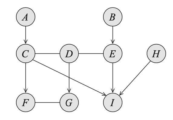
  E.g. node $I$ is a child of nodes $C,E$ and $H$ while $D$ is a parent of $G$.
• If $X_i-X_j\in\mathcal{E}$, we say that $X_i$ is a neighbor of $X_j$, and vice versa.
  E.g. node $F$ is a neighbor of $G$.
• If $X\rightleftharpoons Y\in\mathcal{E}$, we say that $X$ and $Y$ are adjacent.
  E.g. nodes $A$ and $C$ are adjacent, while $D$ is adjacent to $E$.
• We use $\text{Pa}_X$ to denote the set of parents of $X$, $\text{Ch}_X$ to denote the set of its children and $\text{Nb}_X$ to denote its neighbors. The set $\text{Boundary}_X\doteq\text{Pa}_X\cup\text{Nb}_X$ is known as the boundary of $X$.
  E.g. $\text{Pa}_I=\{C,E,H\}$ and $\text{Boundary}_F=\text{Pa}_F\cup\text{Nb}_F=\{C\}\cup\{G\}=\{C,G\}$.
• The degree of a node $X$ is the number of edges in which it participates; its indegree is the number of directed edges $Y\rightarrow X$. The degree of a graph is the maximal degree of a node in the graph.
  E.g. node $D$ has degree of $3$, indegree of $0$; the graph $\mathcal{K}$ has degree of $3$.

Subgraphs

Consider the graph $\mathcal{K}=(\mathcal{X},\mathcal{E})$ and let $\mathbf{X}\subset\mathcal{X}$ be a subset of nodes in $\mathcal{K}$. Then:

• The induced subgraph of $\mathcal{K}$, denoted $\mathcal{K}[\mathbf{X}]$ is defined as the graph $(\mathbf{X},\mathcal{E}')$ where \begin{equation} \mathcal{E}'=\{X\rightleftharpoons Y:X,Y\in\mathbf{X}\} \end{equation}
• A subgraph over $\mathbf{X}$ is complete if every two nodes in $\mathbf{X}$ are connected via some edges. The set $\mathbf{X}$ is known as a clique; or even a maximal clique if for any set of nodes $\mathbf{Y}\supset\mathbf{X}$, $\mathbf{Y}$ is not a clique, i.e. \begin{equation} \{\mathbf{Y}\text{ clique}:\mathbf{Y}\supset\mathbf{X}\}=\emptyset \end{equation}
• The set $\mathbf{X}$ is called upward closed in $\mathbf{K}$ if for any $X\in\mathbf{X}$, we have that \begin{equation} \text{Boundary}_X\subset\mathbf{X} \end{equation} The upward closure of $\mathbf{X}$ is the minimal closed subset $\mathbf{Y}$ covering $\mathbf{X}$, i.e. \begin{equation} \mathbf{Y}=\sup\{\bar{\mathbf{Y}}\text{ upward closed in }\mathcal{K}:\bar{\mathbf{Y}}\supset\mathbf{X}\} \end{equation} The upwardly closed subgraph of $\mathbf{X}$, denoted $\mathcal{K}^+[\mathbf{X}]$, is the induced subgraph over $\mathbf{Y}$, $\mathcal{K}[\mathbf{Y}]$.

Paths, Trails

Consider the graph $\mathcal{K}=(\mathcal{X},\mathcal{E})$, the basic notion of edges gives rise to following definitions:

• $X_1,\ldots,X_k$ form a path in $\mathcal{K}$ if for every $i=1,\ldots,k-1$, we have that either $X_i\rightarrow X_{i+1}$ or $X_i-X_{i+1}$. A path is directed if there exists a directed edge $X_i\rightarrow X_{i+1}$.
• $X_1,\ldots,X_k$ form a trail in $\mathcal{K}$ if for every $i=1,\ldots,k-1$, we have that $X_i\rightleftharpoons X_{i+1}$.
• $\mathcal{K}$ is connected if for every pair $X_i,X_j$ there is a trail between $X_i$ and $X_j$.
• $X$ is an ancestor of $Y$ and correspondingly $Y$ is a descendant of $X$ in $\mathcal{K}$ if there exists a directed path $X_1,\ldots,X_k$ with $X_1=X$ and $X_k=Y$.
• An ordering of nodes $X_1,\ldots,X_n$ is a topological ordering relative to $\mathbf{K}$ if whenever we have $X_i\rightarrow X_j\in\mathcal{E}$, then $i\lt j$. This gives rise to critical results that for each node $X_i$, we have that \begin{equation} \text{Pa}_{X_i}\subset\{X_1,\ldots,X_{i-1}\}, \end{equation} and \begin{equation} \text{Ch}_{X_i}\subset\{X_{i+1},\ldots,X_n\} \end{equation}

Cycles, Loops

• A cycle in $\mathcal{K}$ is a directed path $X_1,\ldots,X_k$ where $X_1=X_k$. $\mathcal{K}$ is acyclic if it contains no cycles.
• $\mathcal{K}$ is a directed acyclic graph (or DAG) if it is both directed and acyclic.
• An acyclic graph containing both directed and undirected edges is known as a partially directed acyclic graph (or PDAG).
  Let $\mathcal{K}$ be a PDAG over $\mathcal{X}$ and let $\mathbf{K}_1,\ldots,\mathbf{K}_\ell$ be a disjoint partition of $\mathcal{X}$ such that:
  • the induced subgraph over $\mathbf{K}_i$ contains no directed edges;
  • for any pair of nodes $X\in\mathbf{K}_i$ and $Y\in\mathbf{K}_j$ for $i\lt j$, an edge between $X$ and $Y$ can only be a directed edge $X\rightarrow Y$.
  Each component $\mathbf{K}_i$ is called a chain component, while $\mathcal{K}$ is referred as a chain graph.
• A loop in $\mathcal{K}$ is a trail $X_1,\ldots,X_k$ where $X_1=X_k$. A graph is singly connected if it contains no loops. A node in a singly connected graph is called a leaf if it has exactly one adjacent node.
• A singly connected directed graph is called a polytree, while a singly connected undirected graph is known as a forest; if it is also connected, it is called a tree.
• A directed graph is a forest if each node has at most one parent. A directed forest is a tree if it is also connected.
• Let $X_1-\ldots-X_k-X_1$ be a loop in the graph, a chord in the loop is an edge connecting two nonconsecutive nodes $X_i$ and $X_j$. An undirected graph $\mathcal{H}$ is known as chordal if any loop $X_1-\ldots-X_k-X_1$ has a chord for $k\geq 4$. This implies that in a chordal graph, the longest minimal loop (the one has no shortcut) has length of $3$.

Directed Graphical Model

A Directed Graphical Model (or Bayesian network) is a tuple $\mathcal{B}=(\mathcal{G},P)$ where

• $\mathcal{G}$ is a Bayesian network structure,
• $P$ factorizes according to $\mathcal{G}$,
• $P$ is specified as a set of CPDs associated with $\mathcal{G}$’s nodes.

Bayesian Network Structure

A Bayesian network structure (or Bayesian network graph, BN graph) is a DAG, denoted $\mathcal{G}=(\mathcal{X},\mathcal{E})$ with $\mathcal{X}=\{X_1,\ldots,X_n\}$ where

• Each node $X_i\in\mathcal{X}$ represents a random variable.
• Each node $X_i\in\mathcal{X}$ is associated with a conditional independencies assumption, called local independencies, denoted $\mathcal{I}_\ell(\mathcal{G})$, which says that $X_i$ is conditionally independent of its non-descendants given its parent, i.e. \begin{equation} (X_i\perp\text{NonDescendants}_{X_i}\vert\hspace{0.1cm}\text{Pa}_{X_i}), \end{equation} where $\text{NonDescendants}_{X_i}$ denotes the set of non-descendant nodes of $X_i$.

I-Maps

Let $P$ be a distribution over $\mathcal{X}$, we define $\mathcal{I}(P)$ to be the set of independence assertions of the form $(X\perp Y\hspace{0.1cm}\vert Z)$ that hold in $P$, i.e. \begin{equation} P\models(X\perp Y\vert Z), \end{equation} or \begin{equation} P(X,Y\vert Z)=P(X\vert Z)P(Y\vert Z) \end{equation} Let $\mathcal{K}$ be a graph associated with a set of independencies $\mathcal{I}(\mathcal{K})$, then $\mathcal{K}$ is an I-map (for independence map) for a set of independencies $\mathcal{I}$ if $\mathcal{I}(\mathcal{K})\subset\mathcal{I}$.

Hence, if $P$ satisfies the local dependencies associated with $\mathcal{G}$, we have \begin{equation} \mathcal{I}_\ell(\mathcal{G})\subset\mathcal{I}(P), \end{equation} which implies that $\mathcal{G}$ is an I-map for $\mathcal{I}(P)$, or simply an I-map for $P$.

Factorization

Let $\mathcal{G}$ is a BN graph over $X_1,\ldots,X_n\in\mathcal{X}$. A distribution $P$ over $\mathcal{X}$ is said to factorize according to $\mathcal{G}$ if $P$ can be expressed as a product \begin{equation} P(X_1,\ldots,X_n)=\prod_{i=1}^{n}P(X_i\vert\text{Pa}_{X_i}) \end{equation} This equation is known as the chain rule for Bayesian networks. Each individual factor $P(X_i\vert\text{Pa}_{X_i})$, which is a conditional probability distribution (CPD), is called the local probabilistic model.

I-Map - Factorization Connection

Theorem 1: Let $\mathcal{G}$ be a BN graph over a set of random variables $\mathcal{X}$ and let $P$ be a joint distribution over $\mathcal{X}$. Then $\mathcal{G}$ is an I-map for $P$ if and only if $P$ factorizes over $\mathcal{G}$.

Proof

• I-map $\Rightarrow$ Factorization
  Without loss of generality, let $X_1,\ldots,X_n$ be a topological ordering of the variables in $\mathcal{X}$.
  Let us consider an arbitrary $X_i$ for $i\in\{1,\ldots,n\}$. As mentioning above, the topological ordering implies that \begin{align} \text{Pa}_{X_i}&\subset\{X_1,\ldots,X_{i-1}\}, \\ \text{Ch}_{X_i}&\subset\{X_{i+1},\ldots,X_n\} \end{align} Consequently, none of descendants of $X_i$ is in $\{X_1,\ldots,X_{n-1}\}$. Thus, if we denote the set of all non-descendant nodes of $X_i$ as $\text{NonDescentdants}_{X_i}$ and let $\mathbf{Z}\subset\text{NonDescentdants}_{X_i}$, then \begin{equation} \mathbf{Z}\cup\text{Pa}_{X_i}=\{X_1,\ldots,X_{i-1}\} \end{equation} Moreover, the local independence for $X_i$ implies that \begin{equation} (X_i\perp\mathbf{Z}\vert\text{ Pa}_{X_i}) \end{equation} Therefore, since $\mathcal{G}$ is an I-map for $P$ we obtain \begin{equation} P(X_i\vert X_1,\ldots,X_{i-1})=P(X_i\vert\text{Pa}_{X_i}) \end{equation} Thus, by the chain rule for probabilities, we have \begin{equation} P(X_1,\ldots,X_n)=\prod_{i=1}^{n}P(X_i\vert X_1,\ldots,X_{i-1})=\prod_{i=1}^{n}P(X_i\vert\text{Pa}_{X_i}) \end{equation}
• I-map $\Leftarrow$ Factorization
  To prove that $\mathcal{G}$ is an I-map according to $P$, we need to show that $\mathcal{I}_\ell(\mathcal{G})$ holds in $P$. Consider an arbitrary node $X_i$ and the local independencies $(X_i\perp\text{NonDescendants}_{X_i}\vert\text{Pa}_{X_i})$, our problem remains to prove that \begin{equation} P(X_i\vert\mathcal{X}\backslash X_i)=P(X_i\vert\text{Pa}_{X_i}) \end{equation} since \begin{equation} P(X_i\vert\mathcal{X}\backslash X_i)=P(X_i\vert\text{NonDescendants}_{X_i}\cup\text{Pa}_{X_i}) \end{equation} By factorization, we have that \begin{align} P(\mathcal{X}\backslash X_i)&=\sum_{X_i}P(X_1,\ldots,X_n) \\ &=\sum_{X_i}\prod_{j=1}^{n}P(X_j\vert\text{Pa}_{X_j}) \\ &=\left(\prod_{j=1,j\neq i}^{n}P(X_j\vert\text{Pa}_{X_j})\right)\sum_{X_i}P(X_i\vert\text{Pa}_{X_i}) \\ &=\prod_{j=1,j\neq i}^{n}P(X_j\vert\text{Pa}_{X_j}), \end{align} where in the last step, we use the fact that the conditional probability function $P(X_i\vert\text{Pa}_{X_i})$ sum to $1$ over the sample space of $X_i$. This implies that by Bayes rules \begin{align} P(X_i\vert\mathcal{X}\backslash X_i)&=\frac{P(X_1,\ldots,X_n)}{P(\mathcal{X}\backslash X_i)} \\ &=\frac{\prod_{j=1}^{n}P(X_j\vert\text{Pa}_{X_j})}{\prod_{j=1,j\neq i}^{n}P(X_j\vert\text{Pa}_{X_j})} \\ &=P(X_i\vert\text{Pa}_{X_i}) \end{align}

Independencies in Bayesian Network

D-separation

Let $\mathcal{G}$ be a BN structure, $X_1\rightleftharpoons\ldots\rightleftharpoons X_n$ be a trail in $\mathcal{G}$ and let $\mathbf{Z}$ be a subset of observed variables. The trail $X_1\rightleftharpoons\ldots\rightleftharpoons X_n$ is active if

• Whenever we have a v-structure $X_{i-1}\rightarrow X_i\leftarrow X_{i+1}$, $X_i$ or one of its descendants are in $\mathbf{Z}$;
• No other node along the trail are in $\mathbf{Z}$.

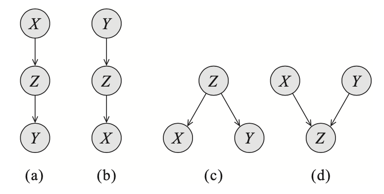
Consider the trails forming from two edges as illustrated above:

• The trail $X\rightarrow Z\rightarrow Y$ is active $\Leftrightarrow$ $Z$ is not observed.
• The trail $X\leftarrow Z\leftarrow Y$ is active $\Leftrightarrow$ $Z$ is not observed.
• The trail $X\leftarrow Z\rightarrow Y$ is active $\Leftrightarrow$ $Z$ is not observed.
• The trail $X\rightarrow Z\leftarrow Y$ is active $\Leftrightarrow$ either $Z$ or one of its descendants is observed.

Let $\mathbf{X},\mathbf{Y},\mathbf{Z}$ be sets of nodes in $\mathcal{G}$. Then $\mathbf{X}$ and $\mathbf{Y}$ are said to be d-separated given $\mathbf{Z}$, denoted $\text{d-sep}_\mathcal{G}(\mathbf{X};\mathbf{Y}\vert\mathbf{Z})$, if there is no active trail between any node $X\in\mathbf{X}$ and $Y\in\mathbf{Y}$ given $\mathbf{Z}$.

We define the global Markov independencies associated with $\mathcal{G}$, denoted $\mathcal{I}(\mathcal{G})$, to be the set of all independencies that correspond to d-separation in $\mathcal{G}$ \begin{equation} \mathcal{I}(\mathcal{G})=\big\{(\mathbf{X}\perp\mathbf{Y}\vert\mathbf{Z}):\text{d-sep}_\mathcal{G}(\mathbf{X};\mathbf{Y}\vert\mathbf{Z})\big\} \end{equation}

Soundness, Completeness

Theorem 2 (Soundness of d-separation) If a distribution $P$ factorizes according to $\mathcal{G}$, then \begin{equation} \mathcal{I}(\mathcal{G})\subset\mathcal{I}(P) \end{equation} The soundness property says that if $\text{d-sep}_\mathcal{G}(X;Y\vert\mathbf{Z})$ then they are conditional independent given $\mathbf{Z}$, or $(X\perp Y\vert\mathbf{Z})$.

Theorem 3 (Completeness of d-separation) If two variables $X$ and $Y$ are independent given $\mathbf{Z}$, then they are d-separated.

The completeness property says that d-separation detects all possible independencies.

Theorem 4: Let $\mathcal{G}$ be a BN graph. If $X$ and $Y$ are not d-separated given $\mathbf{Z}$, then $X$ and $Y$ are dependent given $\mathbf{Z}$ in some distribution $P$ that factorizes over $\mathcal{G}$.

Theorem 5: For almost all distributions $P$ that factorize over $\mathcal{G}$, i.e. for all distributions except for a set of measure zero in the space of CPD parameterizations, we have that \begin{equation} \mathcal{I}(\mathcal{G})=\mathcal{I}(P) \end{equation} These results state that for almost all parameterizations $P$ of the graph $\mathcal{G}$, the d-separation test precisely characterizes the independencies that hold for $P$.

I-Equivalence

Two graph $\mathcal{K}_1$ and $\mathcal{K}_2$ over $\mathcal{X}$ are said to be I-equivalent if they encode the same set of conditional independencies assertions, i.e. \begin{equation} \mathcal{I}(\mathcal{K}_1)=\mathcal{I}(\mathcal{K}_2) \end{equation} This implies that any distribution $P$ that factorizes over $\mathcal{K}_1$ also factorizes according to $\mathcal{K}_2$ and vice versa.

The skeleton of a BN graph $\mathcal{G}$ over $\mathcal{X}$ is an undirected graph over $\mathcal{X}$ containing an edge $\{X,Y\}$ for every edge $(X,Y)$ in $\mathcal{G}$.

Theorem 6 (skeleton + v-structures $\Rightarrow$ I-equivalence) Let $\mathcal{G}_1$ and $\mathcal{G_2}$ be two graphs over $\mathcal{X}$. If $\mathcal{G}_1,\mathcal{G}_2$ both have the same skeleton and the same set of v-structures then they are I-equivalent.²

Immorality

A v-structure $X\rightarrow Z\leftarrow Y$ is an immorality if there is no direct edge between. If there is such an edge, it is called a covering edge for the v-structure.

It is easily seen that not every v-structure is an immorality, which implies that two networks with the same set of immoralities do not necessarily have the same set of v-structures.

Theorem 7 (skeleton + immoralities $\Leftrightarrow$ I-equivalence) Let $\mathcal{G}_1$ and $\mathcal{G_2}$ be two graphs over $\mathcal{X}$. If $\mathcal{G}_1,\mathcal{G}_2$ both have the same skeleton and the same set of immoralities iff they are I-equivalent.

Proof

• To prove the theorem, we first introduce the notion of minimal active trail and triangle.
  Definition (Minimal active trail) An active trail $X_1,\ldots,X_m$ is minimal if there is no other active trail from $X_1$ to $X_m$ that shortcuts some of the nodes, i.e. there is no active trail \begin{equation} X_1\rightleftharpoons X_{i_1}\rightleftharpoons\ldots X_{i_k}\rightleftharpoons X_m\hspace{1cm}\text{for }1\lt i_1\lt\ldots\lt i_k\lt m \end{equation} Definition (Triangle) Any three consecutive nodes in a trail $X_1,\ldots,X_m$ are called a triangle if their skeleton is fully connected, i.e. forms a 3-clique.
  
  Our attention now is to prove that the only possible triangle in minimal active trail is the one having form of $X_{i-1}\leftarrow X_i\rightarrow X_{i+1}$ and either $X_{i-1}\rightarrow X_{i+1}$ or $X_{i-1}\leftarrow X_{i+1}$.
  Consider a two-edge trail from $X_{i-1}$ to $X_{i+1}$ via $X_i$, which as being mentioned above, has four possible forms
  • $X_{i-1}\rightarrow X_i\rightarrow X_{i+1}$
    It is easily seen that $X_i$ has to be not observed to make the trail active. If $X_{i-1}$ is connected to $X_{i+1}$ via $X_{i-1}\rightarrow X_{i+1}$, this gives rise to a shortcut. On the other hand, if they are connected by $X_{i-1}\leftarrow X_{i+1}$, the triangle now induces a cycle.
  • $X_{i-1}\leftarrow X_i\leftarrow X_{i+1}$
    This case is symmetrically identical to the previous one, and thus is not viable.
  • $X_{i-1}\leftarrow X_i\rightarrow X_{i+1}$
    The first observation is that $X_i$ has to be not given. The second observation is $X_{i-1}$ and $X_{i+1}$ are symmetric through $X_i$, so we only need to consider some specific cases of $X_{i-1}$ and the same logic is applied to $X_{i+1}$ analogously.
    Let us examine the two-edge trail $X_{i-2},X_{i-1},X_i$. On the one hand, if we have $X_{i-2}\rightarrow X_{i-1}$, $X_{i-1}$ then has to be given, which implies that
    • If $X_{i-1}\leftarrow X_{i+1}$ exists, it will create a shortcut, which is not allowed.
    • If $X_{i-1}\rightarrow X_{i+1}$ exists, no shortcut appears, $X_{i-1},X_i,X_{i+1}$ satisfies the condition of a triangle in the minimal active trail $X_1,\ldots,X_m$.
    On the other hand, if we have $X_{i-2}\leftarrow X_{i-1}$, then $X_{i-1}$ is not observed, analogously, we instead have
    • If $X_{i-1}\leftarrow X_{i+1}$ exists, no shortcut is formed, $X_{i-1},X_i,X_{i+1}$ create a triangle.
    • If $X_{i-1}\rightarrow X_{i+1}$ exists, $X_{i-1},X_i,X_{i+1}$ is do not form a triangle due to the appearance of a shortcut through $X_{i-1}$ to $X_{i+1}$.
  • $X_{i-1}\rightarrow X_i\leftarrow X_{i+1}$
    In this case, $X_i$ or one of its descendant is observed. Using the similar procedure to previous case gives us no viable triangle formed by $X_{i-1},X_i,X_{i+1}$.
  Given these results, we are now ready for the main part. Let us begin with the forward path.
• Skeleton + Immoralities $\Rightarrow$ I-equivalence
  Assume that there exists node $X,Y,Z$ such that \begin{align} (X\perp Y\vert Z)&\in\mathcal{I}(\mathcal{G}_1), \\ (X\perp Y\vert Z)&\not\in\mathcal{I}(\mathcal{G}_2), \end{align} which implies that there is an active trail through $X,Y$ and $Z$ in the graph $\mathcal{G}_2$. Let us consider the minimal one and continue by examining two cases that whether $Z$ is observed.
  • If $Z$ is observed, in $\mathcal{G}_1$, we have $X\rightarrow Z\rightarrow Y$, or $X\leftarrow Z\leftarrow Y$, or $X\leftarrow Z\rightarrow Y$, while we have $X\rightarrow Z\leftarrow Y$ in $\mathcal{G}_2$, which is a v-structure. To assure that both graphs have the same set of moralities, there exist an edge that directly connects $X$ and $Y$, or in other words, $X,Y,Z$ form a triangle. This contradicts to the claim we have proved in the previous part.
  • If $Z$ is not observed, thus in $\mathcal{G}_1$, $X,Y,Z$ now must form a v-structure $X\rightarrow Z\leftarrow Y$. And also, to guarantee that both graphs have the same moralities, there exists an edge, without loss of generality, we assume $X\rightarrow Y$. However, this edge will active the trail $X,Y,Z$, or in other words, in $\mathcal{G}_1$, we now have $(X\not\perp Y\vert Z)$, which is a contradiction of our assumption.
• Skeleton + Immoralities $\Leftarrow$ I-equivalence
  Consider two I-equivalent graphs $\mathcal{G}_1$ and $\mathcal{G}_2$.
  • First assuming that they do not have that same skeleton. This implies without loss of generality that there exists a trail in $\mathcal{G}_1$ that does not appear in $\mathcal{G}_2$, which induces a conditional independence in $\mathcal{G}_1$ but not in $\mathcal{G}_2$, contradicts to the fact that they two graphs are I-equivalent.
  • Now assuming that two graphs do not have the same set of moralities.

From Distributions to Graphs

Given a distribution $P$, how can we represent the independencies of $P$ with a graph $\mathcal{G}$?

Minimal I-Maps

A graph $\mathcal{K}$ is a minimal I-map for a set of independencies $\mathcal{I}$ if it is an I-map for $\mathcal{I}$, and removing one edge from $\mathcal{K}$ makes it no longer be an I-map.

Perfect Maps

A graph $\mathcal{K}$ is a perfect map (or P-map) for a set of independencies $\mathcal{I}$ if we have that $\mathcal{I}(\mathcal{K})=\mathcal{I}$; and if $\mathcal{I}(\mathcal{K})=\mathcal{I}(P)$, $\mathcal{K}$ is said to be a perfect map for $P$.

Undirected Graphical Model

Similar to the directed case, each node in an undirected graphical model represents a random variable. However, as indicated from the name, each edge that connects two nodes is now undirected, and thus can not describe causal relationship between those nodes as in Bayesian network.

Markov Networks

Factors

Let $\mathbf{D}$ be a set of r.v.s. The function $\phi:\text{Val}(\mathbf{D})\mapsto\mathbb{R}$ is referred as a factor with the scope $\mathbf{D}$, denoted $\mathbf{D}=\text{Scope}(\phi)$.

A factor is nonnegative if all of its entries are nonnegative.

Let $\mathbf{X},\mathbf{Y},\mathbf{Z}$ be disjoint sets of variables, and let $\phi_1(\mathbf{X},\mathbf{Y})$ and $\phi_2(\mathbf{Y},\mathbf{Z})$ be factors. The product $\phi_1\times\phi_2$ is called a factor product, which is a factor $\psi:\text{Val}(\mathbf{X},\mathbf{Y},\mathbf{Z})\mapsto\mathbb{R}$, given as \begin{equation} \psi(\mathbf{X},\mathbf{Y},\mathbf{Z})=\phi_1(\mathbf{X},\mathbf{Y})\cdot\phi_2(\mathbf{Y},\mathbf{Z}) \end{equation}

It is worth remarking that both CPDs and joint distribution are factors. As each Bayesian network define a joint distribution factor, which is the product of the CPDs factor. Specifically, let $\phi_{X_i}(X_i,\text{Pa}_{X_i})$ denote $P(X\vert\text{Pa}_{X_i})$, we can write \begin{equation} P(X_1,\ldots,X_n)=\prod_{i=1}^{n}\phi_{X_i} \end{equation}

Markov Random Fields

Given the notions of factor and factor product, we are now ready to define an undirected parameterization of a distribution.

An Undirected Graphical Model (or Markov Random Field, or Markov network) is defined by an undirected graph $\mathcal{H}$ and a probability distribution $P_\Phi$ parameterized by a set of factors $\Phi=\{\phi_1(\mathbf{D}_1),\ldots,\phi_K(\mathbf{D}_K)\}$ over variables $X_1,\ldots,X_n$ such that \begin{equation} P_\Phi(X_1,\ldots,X_n)=\frac{1}{Z}\tilde{P}_\Phi(X_1,\ldots,X_n), \end{equation} where

• Each node of $\mathcal{H}$ correspond to a variable $X_i$.
• The factor product \begin{equation} \tilde{P}_\Phi(X_1,\ldots,X_n)=\phi_1(\mathbf{D}_1)\times\ldots\times\phi_K(\mathbf{D}_K) \end{equation} is an unnormalized measure.
• $Z$ is a normalizing constant called the partition function, given by \begin{equation} Z=\sum_{X_1,\ldots,X_n}\tilde{P}_\Phi(X_1,\ldots,X_n) \end{equation}
• $P_\Phi$ is also called a Gibbs distribution, which factorizes over $\mathcal{H}$, in the sense that each $\mathbf{D}_k$ for $k=1,\ldots,K$ is a complete subgraph (or clique) of $\mathcal{H}$.
• The factors $\phi_1,\ldots,\phi_K$ that parameterize $\mathcal{H}$ are referred as clique potentials, or potential functions of $\mathcal{H}$.

Reduced Markov Networks

Consider the task of conditioning a distribution on some assignment $\mathbf{u}$ to some subset of variables $\mathbf{U}$. This task corresponds to the process

• Step 1. Eliminate all entries in the joint distribution that are inconsistent with the event $\mathbf{U}=\mathbf{u}$.
• Step 2. Normalize the remaining entries to sum to $1$.

Consider the case that the distribution is in form of $P_\Phi$ for some set of factor $\Phi$.

Factor Reduction

Let $\phi(\mathbf{Y})$ be a factor, and let $\mathbf{U}=\mathbf{u}$ be an assignment for $\mathbf{U}\subset\mathbf{Y}$. The reduction of the factor $\phi$ to the context $\mathbf{U}=\mathbf{u}$, denoted $\phi[\mathbf{U}=\mathbf{u}]$, or $\phi[\mathbf{u}]$ for short, is defined to be a factor over scope $\mathbf{Y}’=\mathbf{Y}\backslash\mathbf{U}$, such that \begin{equation} \phi[\mathbf{u}](\mathbf{y}’)=\phi(\mathbf{y}’,\mathbf{u}) \end{equation} For $\mathbf{U}\not\subset\mathbf{Y}$, we define $\phi[\mathbf{u}]$ to be $\phi[\mathbf{U}’=\mathbf{u}’]$ where

• $\mathbf{U}’=\mathbf{U}\cap\mathbf{Y}$;
• $\mathbf{u}’\doteq\mathbf{u}[\mathbf{U}’]$, where $\mathbf{u}[\mathbf{U}’]$ denotes the assignment in $\mathbf{u}$ to the variable in $\mathbf{U}’$.

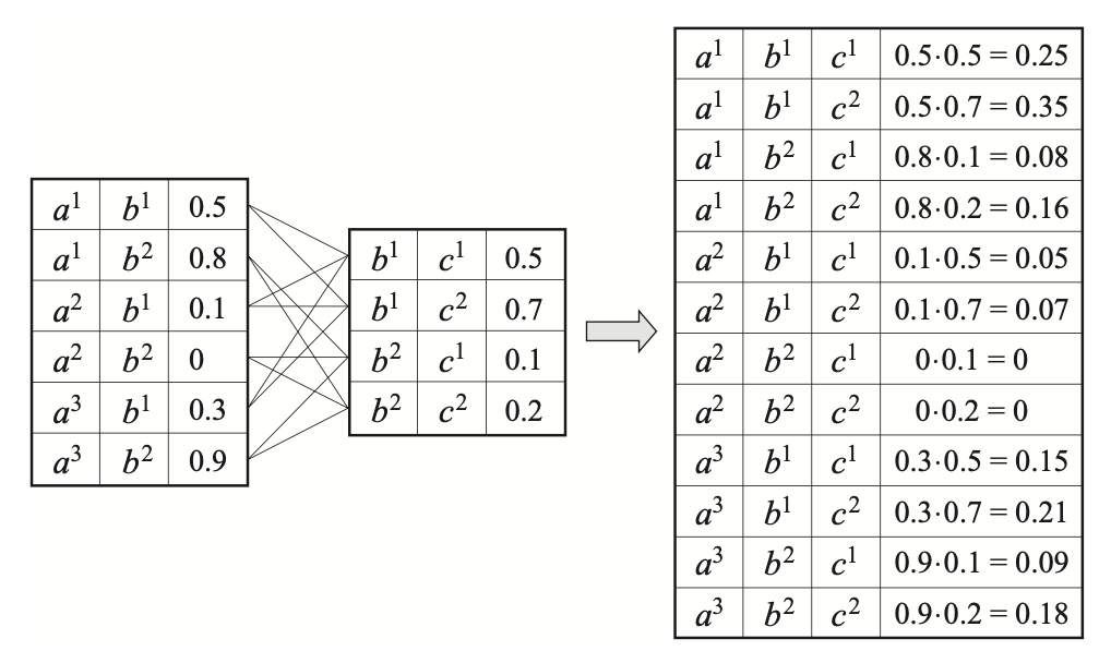
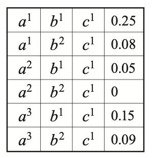
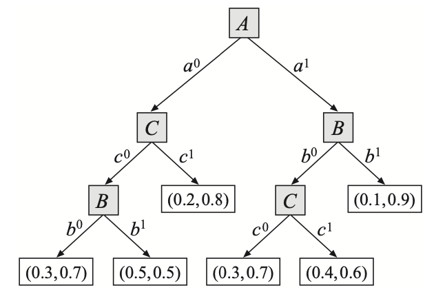
Example 1: Consider the factor $\phi$ with $\text{Scope}(\phi)=\{A,B,C\}$, as given in the right-most table of Figure 4. The reduction of $\phi$ to the context $C=c^1$ is a factor over scope $\{A,B,C\}\backslash\{C\}=\{A,B\}$, given by \begin{equation} \phi[c^1](a,b)=\phi(a,b,c^1), \end{equation} which is illustrated in the following table

With the definition of factor reduction, let us consider a product of factors. We have that an entry in the product is consistent with $\mathbf{u}$ iff it is a product of entries that are all consistent with $\mathbf{u}$.

Reduced Gibbs Distribution

Let $P_\Phi$ be a Gibbs distribution parameterized by $\Phi=\{\phi_1,\ldots,\phi_K\}$, and let $\mathbf{u}$ be a context. The reduced Gibbs distribution $P_\Phi[\mathbf{u}]$ is the Gibbs distribution defined by the set of factors \begin{equation} \Phi[\mathbf{u}]=\{\phi_1[\mathbf{u}],\ldots,\phi_K[\mathbf{u}]\} \end{equation}

Proposition 8: Let $P_\Phi(\mathbf{X})$ be a Gibbs distribution, we then have \begin{equation} P_\Phi[\mathbf{u}]=P_\Phi(\mathbf{W}\vert\mathbf{u}), \end{equation} where $\mathbf{W}=\mathbf{X}\backslash\mathbf{U}$.

Reduced Markov Network

Let $\mathcal{H}$ be a Markov network over the nodes $\mathbf{X}$ and $\mathbf{U}=\mathbf{u}$ be a context. The reduced Markov network $\mathcal{H}[\mathbf{u}]$ is a Markov network over the nodes $\mathbf{W}=\mathbf{X}\backslash\mathbf{U}$, where we have an edge $X-Y$ if there is an edge $X-Y$ in $\mathcal{H}$.

Proposition 9: Let $P_\Phi(\mathbf{X})$ be a Gibbs distribution that factorizes over $\mathcal{H}$, and let $\mathbf{U}=\mathbf{u}$ be a context. Then we have that $P_\Phi[\mathbf{u}]$ factorizes over $\mathcal{H}[\mathbf{u}]$.

Independencies in Markov Network

Analogy to Bayesian network, the graph structure in a Markov Random Field can be viewed as encoding a set of independence assumptions, which can be specified by considering the undirected paths through nodes.

Separation

Let $\mathcal{H}$ be a Markov network structure and let $X_1-\ldots-X_k$ be a path in $\mathcal{H}=(\mathcal{X},\mathcal{E})$. Let $\mathbf{Z}\subset\mathcal{X}$ be a set of observed variables. Then $X_1-\ldots-X_k$ is active given $\mathbf{Z}$ if none of $X_1,\ldots,X_k$ is in $\mathbf{Z}$.

Let $\mathbf{X},\mathbf{Y}$ be set of nodes in $\mathcal{H}$. We say that $\mathbf{Z}$ separates $\mathbf{X}$ and $\mathbf{Y}$, denoted $\text{sep}_\mathcal{H}(\mathbf{X};\mathbf{Y}\vert\mathbf{Z})$ if there is no active path between any node $X\in\mathbf{X}$ and $Y\in\mathbf{Y}$ given $\mathbf{Z}$.

Global Markov Independencies

As in the case of Bayesian network, we define the global Markov independencies associated with $\mathcal{H}$, denoted $\mathcal{I}(\mathcal{H})$, to be the set of all independencies correspond to separation in $\mathcal{H}$ \begin{equation} \mathcal{I}(\mathcal{H})=\big\{(\mathbf{X}\perp\mathbf{Y}\vert\mathbf{Z}):\text{sep}_\mathcal{H}(\mathbf{X};\mathbf{Y}\vert\mathbf{Z})\big\} \end{equation}

Local Markov Independencies

Let $\mathcal{H}$ be a Markov network. We define the pairwise independencies associated with $\mathcal{H}$ to be \begin{equation} \mathcal{I}_p(\mathcal{H})=\big\{(X\perp Y\vert\mathcal{X}\backslash\{X,Y\}):X-Y\notin\mathcal{H}\big\} \end{equation} Or in other words, the pairwise independencies states that $X$ and $Y$ are independent given all other nodes in $\mathcal{H}$.

For a given graph $\mathcal{H}$ and for an arbitrary node $X$ of $\mathcal{H}$, the set of neighbors of $X$ is also called the Markov blanket of $X$, denoted $\text{MB}_\mathcal{H}(X)$. With this notion, we define the local independencies, or Markov local independencies, associated with $\mathcal{H}$ to be \begin{equation} \mathcal{I}_\ell(\mathcal{H})=\big\{\big(X\perp\mathcal{X}\backslash(\{X\}\cup\text{MB}_\mathcal{H}(X))\vert\text{MB}_\mathcal{H}(X)\big):X\in\mathcal{X}\big\} \end{equation} Or in other words, the Markov local independencies says that $X$ is independent of the rest of the nodes in $\mathcal{H}$ given its neighbors.

The definition of Markov blanket can also be rewritten using independencies assertions:
A set $\mathbf{U}$ is a Markov blanket of $X$ in a distribution $P$ if $X\notin\mathbf{U}$ and if $\mathbf{U}$ is a minimal set of nodes such that \begin{equation} \big(X\perp\mathcal{X}\backslash(\{X\}\cup\mathbf{U})\vert\mathbf{U}\big)\in\mathcal{I}(P) \end{equation}

Markov Independencies Relationships

Theorem 10: Let $\mathcal{H}$ be a Markov network and $P$ be a positive distribution. The following three statement are then equivalent:

• $P\models\mathcal{I}_\ell(\mathcal{H})$.
• $P\models\mathcal{I}_p(\mathcal{H})$.
• $P\models\mathcal{I}(\mathcal{H})$.

Proof

• (i) $\Rightarrow$ (ii)
  Consider an arbitrary node $X$ in $\mathcal{H}$. Let $Y\in\mathcal{X}$ such that $X-Y\notin\mathcal{H}$, then $Y\notin\text{MB}_\mathcal{H}(X)$, or in other words \begin{equation} Y\in\mathcal{X}\backslash(\{X\}\cup\text{MB}_\mathcal{H}(X)) \end{equation} Moreover, since $P\models\mathcal{I}_\ell(\mathcal{H})$, we have that $P$ satisfies \begin{equation} \big(X\perp\mathcal{X}\backslash(\{X\}\cup\text{MB}_\mathcal{H}(X))\vert\text{MB}_\mathcal{H}(X)\big), \end{equation} which implies that \begin{equation} \big(X\perp Y\vert\text{MB}_\mathcal{X}\cup\mathcal{X}\backslash(\{X,Y\}\cup\text{MB}_\mathcal{H}(X))\big) \end{equation} holds for $P$. Or in other words, for any $X,Y$ such that $X-Y\notin\mathcal{H}$, we have \begin{equation} P\models(X\perp Y\vert\mathcal{X}\backslash\{X,Y\}), \end{equation} which proves our claim.
• (ii) $\Rightarrow$ (iii)
• (iii) $\Rightarrow$ (i)
  This follows directly from the fact that if two nodes $X$ and $Y$ are not connected, then they are necessarily separated by all remaining nodes of the graph.

Soundness, Completeness

Theorem 11 (Soundness of separation) Let $\mathcal{H}=(\mathcal{X},\mathcal{E})$ be a Markov network structure and let $P$ be a distribution over $\mathcal{X}$. If $P$ is a Gibbs distribution that factorizes over $\mathcal{H}$, then $\mathcal{H}$ is an I-map for $P$.

Proof
Let $\mathbf{X},\mathbf{Y}$ and $\mathbf{Z}$ be any disjoint subsets of $\mathcal{X}$ such that $\text{sep}_\mathcal{H}(\mathbf{X};\mathbf{Y}\vert\mathbf{Z})$. We need to show that \begin{equation} P\models(\mathbf{X}\perp\mathbf{Y}\vert\mathbf{Z}) \end{equation} We begin by considering the case that $\mathbf{X}\cup\mathbf{Y}\cup\mathbf{Z}=\mathcal{X}$. Since $\mathbf{Z}$ separates $\mathbf{X}$ and $\mathbf{Y}$, then for any $X\in\mathbf{X}$ and for any $Y\in\mathbf{Y}$, there is no direct edge between $X,Y$. This implies that any clique in $\mathcal{H}$ is either in $\mathbf{X}\cup\mathbf{Z}$ or in $\mathbf{Y}\cup\mathbf{Z}$.

Let $I_\mathbf{X}$ denote the indices of the set of cliques within $\mathbf{X}\cup\mathbf{Z}$ and let $I_\mathbf{Y}$ represent the indices of the ones in $\mathbf{Y}\cup\mathbf{Z}$. Thus, as $P$ factorizes over $\mathcal{H}$, we have that \begin{align} P(X_1,\ldots,X_n)&=\frac{1}{Z}\prod_{i}\phi_i(\mathbf{D}_i) \\ &=\frac{1}{Z}\left(\prod_{i\in I_\mathbf{X}}\phi_i(\mathbf{D}_i)\right)\cdot\left(\prod_{i\in I_\mathbf{Y}}\phi_i(\mathbf{D}_i)\right) \\ &=\frac{1}{Z}\phi_\mathbf{X}(\mathbf{X},\mathbf{Z})\phi_\mathbf{Y}(\mathbf{Y},\mathbf{Z}), \end{align} where $\phi_\mathbf{X},\phi_\mathbf{Y}$ are some factors with scopes $\mathbf{X}\cup\mathbf{Z}$ and $\mathbf{Y}\cup\mathbf{Z}$ respectively. Hence, it follows that \begin{equation} P\models(\mathbf{X}\perp\mathbf{Y}\vert\mathbf{Z}) \end{equation} Now consider the case that $\mathbf{X}\cup\mathbf{Y}\cup\mathbf{Z}\subset\mathcal{X}$. Let $\mathbf{U}=\mathcal{X}\backslash(\mathbf{X}\cup\mathbf{Y}\cup\mathbf{Z})$. We can divide $\mathbf{U}$ into two disjoint sets $\mathbf{U}_1$ and $\mathbf{U}_2$ such that \begin{equation} \text{sep}_\mathcal{H}(\mathbf{X}\cup\mathbf{U}_1;\mathbf{Y}\cup\mathbf{U}_2\vert\mathbf{Z}) \end{equation} And since $(\mathbf{X}\cup\mathbf{U}_1)\cup(\mathbf{Y}\cup\mathbf{U}_2)\cup\mathbf{Z}=\mathcal{X}$, we can follow the previous procedure to conclude that \begin{equation} P\models(\mathbf{X}\cup\mathbf{U}_1\perp\mathbf{Y}\cup\mathbf{U}_2\vert\mathbf{Z}), \end{equation} which implies that \begin{equation} P\models(\mathbf{X}\perp\mathbf{Y}\vert\mathbf{Z}) \end{equation}

Theorem 12 (Hammersley-Clifford) Let $\mathcal{H}=(\mathcal{X},\mathcal{E})$ be a Markov network structure and let $P$ be a positive distribution over $\mathcal{X}$. If $\mathcal{H}$ is an I-map for $P$, then $P$ is a Gibbs distribution that factorizes over $\mathcal{H}$.

Corollary 13: The positive distribution $P$ factorizes a Markov network $\mathcal{H}$ iff $\mathcal{H}$ is an I-map for $P$.

Theorem 14 (Completeness of separation) Let $\mathcal{H}$ be a Markov network structure. If $X$ and $Y$ are not separated given $\mathbf{Z}$ in $\mathcal{H}$, then $X$ and $Y$ are dependent given $\mathbf{Z}$ in some distribution $P$ that factorizes over $\mathcal{H}$.

From Distributions to Graphs

As mentioned above, the notion of minimal I-map lets us encode the independencies of a given distribution $P$ using a graph structure.

In particular, for a distribution $P$, we can construct the minimal I-map based on either the pairwise independencies or the local independencies.

Theorem 15: Let $P$ be a positive distribution and $\mathcal{H}$ be a Markov network defined by including an edge $X-Y$ for all $X,Y$ such that $P\not\models(X\perp Y\vert\mathcal{X}\backslash\{X,Y\}) $. Then $\mathcal{H}$ is the unique minimal I-map for $P$.

Theorem 16: Let P be a positive distribution and let $\mathcal{H}$ be a Markov network defined by including an edge $X-Y$ for all $X$ and all $Y\in\text{MB}_\mathcal{H}(X)$. Then $\mathcal{H}$ is the unique minimal I-map for $P$.

Remark: Not every distribution has a perfect map as UGM (proof by contradiction).

Factor Graphs

A factor graph $\mathcal{F}$ is an undirected graph whose nodes are divided into two groups: variable nodes (denoted as ovals) and factor nodes (denoted as squares) and whose edges only connect each factor (potential function) $\psi_c$ to its dependent nodes $X\in X_c$.

Log-Linear Models

A distribution $P$ is a log-linear model over a Markov network $\mathcal{H}$ if it is associated with

• a set of features $\mathcal{F}=\{\phi_1(\mathbf{X}_1),\ldots,\phi_k(\mathbf{X}_k)\}$ where each $\mathbf{X}_i$ is a complete subgraph in $\mathcal{H}$,
• a set of weight $w_1,\ldots,w_k$, such that \begin{equation} P(X_1,\ldots,X_n)=\frac{1}{Z}\exp\left[-\sum_{i=1}^{k}w_i\phi_i(\mathbf{X}_i)\right] \end{equation}

The function $\phi_i$ are called energy functions.

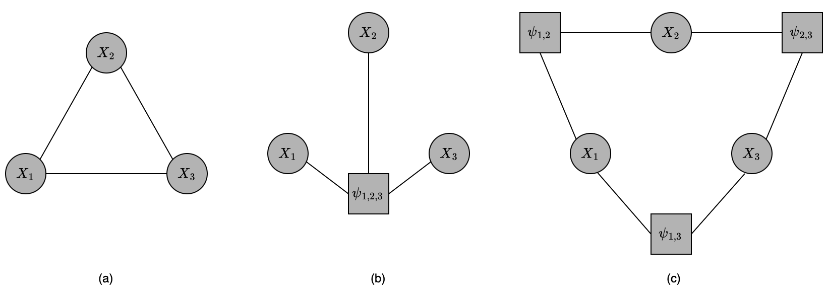
Canonical Parameterization

The canonical parameterization of a Gibbs distribution over $\mathcal{H}$ is defined via a set of energy functions over all cliques. For instance, the Markov network given in Figure 7(a) would have energy functions for each of the cliques \begin{equation} \{\{X_1,X_2,X_3\},\{X_1,X_2\},\{X_2,X_3\},\{X_1,X_3\},\{X_1\},\{X_2\},\{X_3\}\}, \end{equation} plus a constant energy function for the empty clique.

Bayesian & Markov Networks

We are ready to derive the relationship between representations: Bayesian network and Markov network. Specifically, we can find a Bayesian network which is a minimal I-map for a given Markov network and vice versa.

Bayesian Networks to Markov Networks

Let us begin by considering a distribution $P_\mathcal{B}$, where $\mathcal{B}$ is a parameterized network over a graph $\mathcal{G}$. Then, $P_\mathcal{B}$ can be seen as a Gibbs distribution by considering each CPD $P(X_i\vert\text{Pa}_{X_i})$ as a factor with scope $X_i,\text{Pa}_{X_i}$. This Gibbs distribution then has $1$ as its partition function.

Proposition 17: Let $\mathcal{B}$ be a Bayesian network over $\mathcal{X}$ and let $\mathbf{E}=\mathbf{e}$ be an observation. Let $\mathbf{W}=\mathcal{X}\backslash\mathbf{E}$. Then $P_\mathcal{B}(\mathbf{W}\vert\mathbf{e})$ is a Gibbs distribution, defined by the factors $\Phi=\{\phi_{X_i}\}_{X_i\in\mathcal{X}}$, where \begin{equation} \phi_{X_i}=P_\mathcal{B}(X_i\vert\text{Pa}_{X_i})[\mathbf{E}=\mathbf{e}] \end{equation} The partition function for this Gibbs distribution is $P(\mathbf{e})$.

This result lets us consider any Bayesian network conditioned as evidence $\mathbf{e}$ as a Gibbs distribution with partion function $P(\mathbf{e})$.

To find the undirected graph serving as an I-map for a set of factors in a Bayesian network, we recall that we have considered each CPD $P(X_i\vert\text{Pa}_{X_i})$ as a factor with scope $X_i,\text{Pa}_{X_i}$, in the undirected I-map. Therefore, in the undirected I-map, we need to have an edge between $X_i$ and each of its parents, as well as between all of the parents of $X_i$ (due to each factor corresponds to a clique).

Moralized Graph

The moral graph $\mathcal{M}[\mathcal{G}]$ of a Bayesian network structure $\mathcal{G}$ over $\mathcal{X}$ is the undirected graph over $\mathcal{X}$ that consists of an undirected edge between $X$ and $Y$ if

• there is a directed edge between them (in either direction), or
• $X$ and $Y$ are both parents of the same node.

The construction of moral graphs follows directly to a result.

Corollary 18: Let $\mathcal{G}$ be a BN graph. Then for any distribution $P_\mathcal{B}$ such that $\mathcal{B}$ is a parameterization of $\mathcal{G}$, we have that $\mathcal{M}[\mathcal{G}]$ is an I-map for $P_\mathcal{B}$.

Proposition 19: Let $\mathcal{G}$ be any BN graph. The moralized graph $\mathcal{M}[\mathcal{G}]$ is a minimal I-map for $\mathcal{G}$.

Proof
We begin by introducing the notion of Markov blanket in a Bayesian network $\mathcal{G}$.
Definition (Markov blanket in BN) The Markov blanket of a node $X\in\mathcal{X}$ in a Bayesian network $\mathcal{G}$, denoted $\text{MB}_\mathcal{G}(X)$, is the set of $X$’s parents, $X$’s children, and other parents of $X$’s children.

Let $X\in\mathcal{X}$ be a node of $\mathcal{G}$, we have that $\text{MB}_\mathcal{G}(X)$ d-separates $X$ from all other variables in $\mathcal{G}$; and that no subset of $\text{MB}_\mathcal{G}(X)$ has that property. Specifically:

• Let $\mathbf{W}=\mathcal{X}\backslash\big(\{X\}\cup\text{MB}_\mathcal{G}(X)\big)$, and let $Z\in\text{MB}_\mathcal{G}(X)$ be some node in the Markov blanket of $X$. Then for each $Y\in\mathbf{W}$ that connected to $X$ via a trail, we have three possible cases: \begin{equation} X\rightarrow Z\rightarrow Y;X\leftarrow Z\leftarrow Y;X\leftarrow Z\rightarrow Y \end{equation} The v-structure is excluded due to the definition of $\text{MB}_\mathcal{G}(X)$, i.e. if $X\rightarrow Z\leftarrow Y$ exists, then $Y\in\text{MB}_\mathcal{G}(X)$. As $\text{MB}_\mathcal{G}(X)$ is given, $Z$ is observed, all of those 2-edge trails are then in-active, which implies that $\text{d-sep}_\mathcal{G}(X;Y\vert Z)$, and thus $\text{d-sep}_\mathcal{G}(X;\mathbf{W}\vert\text{MB}_\mathcal{G}(X))$.
• As we have mentioned above that if a v-structure exists, then $Y$ must be in the Markov blanket of $X$, it follows directly that $\text{MB}_\mathcal{G}(X)$ is the minimal set having the property.

Thus, in other words, we can conclude that the Markov blanket of $X$, $\text{MB}_\mathcal{G}(X)$, is the smallest set required to render $X$ independent of all other nodes in $\mathcal{G}$. For each $X\in\mathcal{X}$, by viewing its Markov blanket in $\mathcal{G}$ as the set of its neighbors in an undirected graph $\mathcal{H}$ (which is the definition of Markov blanket in a Markov network), we then have that $\mathcal{H}$ is a minimal I-map for $\mathcal{G}$. Additionally, by how it is constructed, $\mathcal{H}$ is also a moral graph of $\mathcal{G}$, and thus $\mathcal{I}(\mathcal{H})\subset\mathcal{I}(\mathcal{G})$.

Remark:

• The addition of the moralizing edges to the Markov network $\mathcal{H}$ leads to the loss of independence information implied by $\mathcal{G}$.
• However, moralization causes loss of independencies assertions only when it introduces new edges into the graph.

Proposition 20: If the directed graph $\mathcal{G}$ is moral (in the sense that it contains no immoralities, i.e. for any pair of $X,Y$ in $\mathcal{G}$ sharing a child, there is a covering edge between $X$ and $Y$), then its moralized graph $\mathcal{M}[\mathcal{G}]$, which now has the same edges as $\mathcal{G}$, is a perfect map of $\mathcal{G}$.

In other words, this result states that a moral graph $\mathcal{G}$ can be converted to a Markov network without losing independencies assertions.

Proof
Let $\mathcal{H}=\mathcal{M}[\mathcal{G}]$, then $\mathcal{H}$ and $\mathcal{G}$ have the same edges. As in Proposition 19, we have shown that $\mathcal{I}(\mathcal{H})\subset\mathcal{I}(\mathcal{G})$, our problem remains to prove that $\mathcal{I}(\mathcal{H})\supset\mathcal{I}(\mathcal{G})$.
Assume that there is an independence \begin{equation} (\mathbf{X}\perp\mathbf{Y}\vert\mathbf{Z})\in\mathcal{I}(\mathcal{G}), \end{equation} which is not in $\mathcal{I}(\mathcal{H})$. This implies that there exists some active trail from $\mathbf{X}$ to $\mathbf{Y}$ given $\mathbf{Z}$ in $\mathcal{H}$. Consider some such trail which is minimal. As $\mathcal{H},\mathcal{G}$ have same edges, the same trail must also exist in $\mathcal{G}$. Thus, it is also in-active in $\mathcal{G}$ given $\mathbf{Z}$, which implies that it contains a v-structure, say $X_1\rightarrow X_2\leftarrow X_3$. Moreover, as $\mathcal{G}$ is moral, there exists an edge connecting $X_1$ and $X_3$, contradicts the assumption that the trail is minimal.

Markov Networks to Bayesian Networks

Theorem 21: Let $\mathcal{H}$ be a Markov network graph, and let $\mathcal{G}$ be any Bayesian network minimal I-map for $\mathcal{H}$. Then $\mathcal{G}$ can have no immoralities.

Chordal Graphs

Theorem 22: Let $\mathcal{H}$ be a non-chordal Markov network. Then there is no Bayesian newtork $\mathcal{G}$ which is a perfect map for $\mathcal{H}$, i.e. $\mathcal{I}(\mathcal{G})=\mathcal{I}(\mathcal{H})$.

Conditional Random Fields

A conditional random field, or CRF, is an undirected graph $\mathcal{H}$ whose nodes correspond to $\mathbf{X}\cup\mathbf{Y}$ where $\mathbf{X}$ is a set of observed variables and $\mathbf{Y}$ is a (disjoint) set of target variables which specifies a conditional distribution (instead of a joint distribution) \begin{equation} P(\mathbf{Y}\vert\mathbf{X})=\frac{1}{Z(\mathbf{X})}\prod_{c\in C}\psi_c(\mathbf{X}_c,\mathbf{Y}_c), \end{equation} where the partition function $Z(\mathbf{X})$ now depends on $\mathbf{X}$ (rather than being a constant) \begin{equation} Z(\mathbf{X})=\sum_\mathbf{Y}\prod_{c\in C}\psi_c(\mathbf{X}_c,\mathbf{Y}_c) \end{equation}

Example - Naive Markov

Consider a CRF over the binary-value variables $\mathbf{X}=\{X_1,\ldots,X_k\}$ and $\mathbf{Y}=\{Y\}$, and a pairwise potential between $Y$ and each $X_i$. The model is referred as a naive Markov model. Assume that the pairwise potentials defined via the log-linear model \begin{equation} \psi_i(X_i,Y)=\exp\big[w_i\mathbf{1}\{X_i=1,Y=1\}\big] \end{equation} Additionally, we also have a single-node potential \begin{equation} \psi_0(Y)=\exp\big[w_0\mathbf{1}\{Y=1\}\big] \end{equation} We then have that \begin{equation} P(Y=1\vert x_1,\ldots,x_k)=\frac{1}{1+\exp\left[-\left(w_0+\sum_{i=1}^{k}w_i x_i\right)\right]} \end{equation}

Local Probabilistic Models

Tabular CPDs

For a space of discrete-valued random variables only, we can encode the CPDs $P(X\vert\text{Pa}_X)$ as a table where each entry corresponds to a pair of $X,\text{Pa}_X$.

It is easily seen that this representation raises a disadvantage that the number of parameters required grows exponentially in the number of parents. Also, it is impossible to store the conditional probability corresponding to a continuous-valued random variables.

To avoid these problems, instead of viewing CPDs as tables listing all of the conditional probabilities $P(x\vert\text{pa}_X)$, we should consider them as functions that given $\text{pa}_X$ and $x$, return the conditional probability $P(x\vert\text{pa}_X)$.

Deterministic CPDs

The simplest type of non-tabular CPD corresponds to a variable $X$ being a deterministic function of its parents $\text{Pa}_X$. It means, there exists $f:\text{Val}(Pa_X)\mapsto\text{Val}(X)$ such that \begin{equation} P(x\vert\text{pa}_X)=\begin{cases}1&\hspace{1cm}x=f(\text{pa}_X) \\ 0&\hspace{1cm}\text{otherwise}\end{cases} \end{equation} Deterministic variables are denoted as double-line ovals, as illustrated in the following example

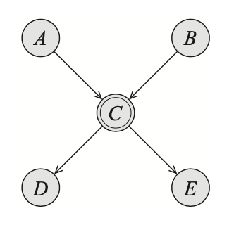
Consider the above figure, as $C$ being a deterministic function of $A$ and $B$, we can deduce that $C$ is fully observed if $A$ and $B$ are both observed. In other words, we have that \begin{equation} (D\perp E\vert A,B) \end{equation}

Theorem 22: Let $\mathcal{G}$ be a network structure, and let $\mathbf{X},\mathbf{Y},\mathbf{Z}$ be sets of variables, $\mathbf{D}$ be set of deterministic variables. If $\mathbf{X}$ is deterministically separated from $\mathbf{Y}$ given $\mathbf{Z}$³, then for all distributions $P$ such that $P\models\mathcal{I}_\ell(\mathcal{G})$ and where, for each $X\in\mathbf{D}$, $P(X\vert\text{Pa}_X)$ is a deterministic CPD, we have that $P\models(\mathbf{X}\perp\mathbf{Y}\vert\mathbf{Z})$.

Theorem 23: Let $\mathcal{G}$ be a network structure, and let $\mathbf{X},\mathbf{Y},\mathbf{Z}$ be sets of variables, $\mathbf{D}$ be set of deterministic variables. If $\mathbf{X}$ is not deterministically separated from $\mathbf{Y}$ given $\mathbf{Z}$, then there exists a distribution $P$ such that $P\models\mathcal{I}_\ell(\mathcal{G})$ and where, for each $X\in\mathbf{D}$, $P(X\vert\text{Pa}_X)$ is a deterministic CPD, but we instead have $P\not\models(\mathbf{X}\perp\mathbf{Y}\vert\mathbf{Z})$.

It is worth remarking that particular deterministic CPD might imply additional independencies. For instance, let us consider the following examples

Example 2: Consider the following Bayesian network

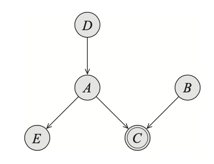
In the above figure, if $C=A\text{ XOR }B$, we have that $A$ is fully determined given $C$ and $B$. In other words, we have that \begin{equation} (D\perp E\vert B,C) \end{equation} Example 3: Consider the network given in Figure 9, with $C=A\text{ OR }B$. Assume that we are given $A=a^1$, it is then immediately that $C=c^1$ without taking into account the value of $B$. Or in other words, we have that \begin{equation} P(D\vert B,a^1)=P(D\vert a^1) \end{equation} On the other hand, given $A=a^0$, the value of $C$ is not fully determined, and still depend the value of $B$.

Context-Specific Independence

Let $\mathbf{X},\mathbf{Y},\mathbf{Z}$ be pairwise disjoint sets of variables, let $\mathbf{C}$ be a set of variable (which might overlap with $\mathbf{X}\cup\mathbf{Y}\cup\mathbf{Z}$), and let $\mathbf{c}\in\text{Val}(\mathbf{C})$. We say that $X$ and $\mathbf{Y}$ are contextually independent given $\mathbf{Z}$ and the context $\mathbf{C}$ denoted $(\mathbf{X}\perp_c\mathbf{Y}\vert\mathbf{Z},\mathbf{c})$ if \begin{equation} P(\mathbf{Y},\mathbf{Z},\mathbf{c})>0\Rightarrow P(\mathbf{X}\vert\mathbf{Y},\mathbf{Z},\mathbf{c})=P(\mathbf{X}\vert\mathbf{Z},\mathbf{c}) \end{equation} Independence statements of this form is known as the context-specific independencies (CSI).

Given this definition, let us examine some examples.

Example 4: Given the Bayesian network in Figure 9 with $C$ being a deterministic function $\text{OR}$ of $A$ and $B$. By properties of $\text{OR}$ function, we can conclude some independence assertions \begin{align} &(C\perp_c B\hspace{0.1cm}\vert\hspace{0.1cm}a^1), \\ &(D\perp_c B\hspace{0.1cm}\vert\hspace{0.1cm}a^1), \\ &(A\perp_c B\hspace{0.1cm}\vert\hspace{0.1cm}c^0), \\ &(D\perp_c E\hspace{0.1cm}\vert\hspace{0.1cm}c^0), \\ &(D\perp_c E\hspace{0.1cm}\vert\hspace{0.1cm}b^0,c^1) \end{align} Example 5: Given the Bayesian network in Figure 10 with $C$ being the exclusive or of $A$ and $B$. We can also conclude some independence assertions using properties of $\text{XOR}$ function \begin{align} &(D\perp_c E\hspace{0.1cm}\vert\hspace{0.1cm}b^1,c^0), \\ &(D\perp_c E\vert\hspace{0.1cm}b^0,c^1) \end{align}

Context-specific CPDs

Tree-CPDs

A tree-CPD representing a CPD for variable $X$ is a rooted tree, where:

• each leaf node is labeled with a distribution $P(X)$;
• each internal node is labeled with some variable $Z\in\text{Pa}_X$;
• each edge from an internal node, which is labeled as some $Z$, to its child nodes corresponds to a $z_i\in\text{Val}(Z)$.

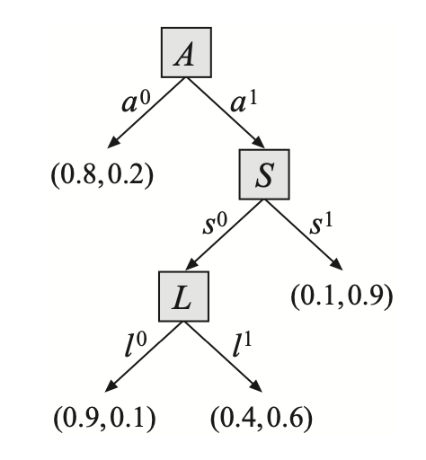
The structure is common in cases where a variable can depend on a set of r.v.s but we have uncertainty about which r.v.s it depends on. For example, in the above tree-CDP representing $P(J\vert A,S,L)$, we have that \begin{align} &(J\perp_c L,S\vert\hspace{0.1cm}a^0), \\ &(J\perp_c L\vert\hspace{0.1cm}a^1,s^1), \\ &(J\perp_c L\vert\hspace{0.1cm}s^1) \end{align}

Multiplexer CPD

A CPD $P(Y\vert A,Z_1,\ldots,Z_k)$ is said to be a multiplexer CPD if $\text{Val}(A)=\{1,\ldots,k\}$ and \begin{equation} P(Y\vert a,Z_1,\ldots,Z_k)=\mathbf{1}\{Y=Z_a\}, \end{equation} where $a$ is the value of $A$. The variable $A$ is referred as the selector variable for the CPD.

Rule CPDs

A rule $\rho$ is a pair $(\mathbf{c},p)$ where $\mathbf{c}$ is an assignment to some subset of variables $\mathbf{C}$ and $p\in[0,1]$. $\mathbf{C}$ is then referred as the scope of $\rho$, denoted $\mathbf{C}=\text{Scope}(\rho)$.

This representation decomposes a tree-CPD into its most basic elements.

Example 6: Consider the tree-CPD given in Figure 11. The tree defines eight rules \begin{equation} \left\{\begin{array}{l}(a^0,j^0;0.8), \\ (a^0,j^1;0.2), \\ (a^1,s^0,l^0,j^0;0.9), \\ (a^1,s^0,l^0,j^1;0.1), \\ (a^1,s^0,l^1,j^0;0.4), \\ (a^1,s^0,l^1,j^1;0.6), \\ (a^1,s^1,j^0;0.1), \\ (a^1,s^1,j^1;0.9)\end{array}\right\} \end{equation} It is necessary that each conditional distribution $P(X\vert\text{Pa}_X)$ is specified by exactly one rule. Or in other words, the rules in a tree-CPD must be mutually exclusive and exhaustive.

Rule-based CPD

A rule-based CPD $P(X\vert\text{Pa}_X)$ is a set of rules $\mathcal{R}$ such that

• For each $\rho\in\mathcal{R}$, we have that \begin{equation} \text{Scope}(\rho)\subset\{X\}\cup\text{Pa}_X \end{equation}
• For each assignment $(x,\mathbf{u})$ to $\{X\}\cup\text{Pa}_X$, we have exactly one rule $(\mathbf{c};p)\in\mathcal{R}$ such that $\mathbf{c}$ is compatible with $(x,\mathbf{u})$. And we say that \begin{equation} P(X=x\vert\text{Pa}_X=\mathbf{u})=p \end{equation}
• $\sum_x P(x\vert\mathbf{u})=1$.

Example 7: Let $X$ be a variable with $\text{Pa}_X=\{A,B,C\}$ with $X$’s CPD is defined by sets of rules \begin{equation} \left\{\begin{array}{l}\rho_1:(a^1,b^1,x^0;0.1), \\ \rho_2:(a^1,b^1,x^1;0.9), \\ \rho_3:(a^0,c^1,x^0;0.2), \\ \rho_4:(a^0,c^1,x^1;0.8), \\ \rho_5:(b^0,c^0,x^0;0.3), \\ \rho_6:(b^0,c^0,x^1;0.7), \\ \rho_7:(a^1,b^0,c^1,x^0;0.4), \\ \rho_8:(a^1,b^0,c^1,x^1;0.6), \\ \rho_9:(a^0,b^1,c^0;0.5)\end{array}\right\} \end{equation} The tree-CPD corresponds to the above rule-based CPD $P(X\vert A,B,C)$ is given as:

It is worth noticing that both CPD entries $P(x^0\vert a^0,b^1,c^0)$ and $P(x^1\vert a^0,b^1,c^0)$ are determined by rule $\rho_9$ only. This kind of rule only works for uniform distribution.

Independencies in Context-specific CPDs

If $\mathbf{c}$ be a context associated with a branch in the tree-CPD for $X$, then $X$ is independent of the remaining parents, $\text{Pa}_X\backslash\text{Scope}(\mathbf{c})$, given $\mathbf{c}$. Moreover, there might exist CSI statements conditioned on contexts which are not induced by complete branches.

Example 8: Consider the tree-CPD given in Figure 11, as mentioned above, we have that \begin{equation} (J\perp_c L\hspace{0.1cm}\vert\hspace{0.1cm}s^1), \end{equation} where $s^1$ is not the full assignment associated with a branch.
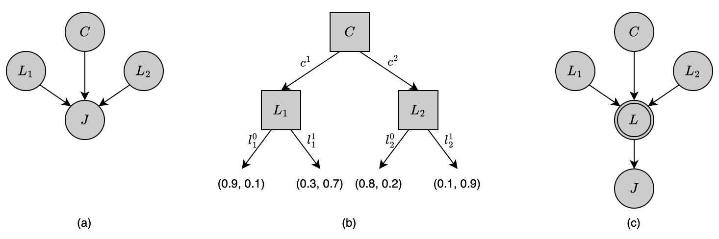
Also, consider the tree-CPD given in Figure 12(b), we have that \begin{align} &(J\perp_c L_2\hspace{0.1cm}\vert\hspace{0.1cm}c^1), \\ &(J\perp_c L_1\hspace{0.1cm}\vert\hspace{0.1cm}c^2), \end{align} where neither $c^1$ nor $c^2$ is the full assignment associated with a branch.

Reduced Rule

Let $\rho=(\mathbf{c}’;p)$ be a rule and $\mathbf{c}$ be a context. If $\mathbf{c}’$ is compatible with $\mathbf{c}$, we say that $\rho\sim\mathbf{c}$.

In this case, let $\mathbf{c}’’$ be the assignment in $c’$ to the variables in $\text{Scope}(\mathbf{c}’)\backslash\text{Scope}(\mathbf{c})$. We then define the reduced rule $\rho[\mathbf{c}]=(\mathbf{c}’’;p)$. If $\mathcal{R}$ be a set of rules, we define the reduced rule set \begin{equation} \mathcal{R}[\mathbf{c}]=\{\rho[\mathbf{c}]:\rho\in\mathcal{R},\rho\sim\mathbf{c}\} \end{equation}

Example 9: Consider the rule set $\mathcal{R}$ given in Example 7, we have that the reduced set corresponding to context $a^1$ is \begin{equation} \mathcal{R}[a^1]=\left\{\begin{array}{l}\rho_1’:(b^1,x^0;0.1), \\ \rho_2:(b^1,x^1;0.9), \\ \rho_5:(b^0,c^0,x^0;0.3), \\ \rho_6:(b^0,c^0,x^1;0.7), \\ \rho_7:(b^0,c^1,x^0;0.4), \\ \rho_8’:(b^0,c^1,x^1;0.6),\end{array}\right\} \end{equation} which is obtained by selecting rules compatible with $a^1$, i.e. $\{\rho_1,\rho_2,\rho_5,\rho_6,\rho_7,\rho_8\}$, then canceling out $a^1$ from all the rules where it appeared.

Proposition 20: Let $\mathcal{R}$ be the rules in the rule-based CPD for a variable $X$, and let $\mathcal{R}_\mathbf{c}$ be the rules in $\mathcal{R}$ compatible with $\mathbf{c}$. Let $\mathbf{Y}\subset\text{Pa}_X$ be a subset such that $\mathbf{Y}\cap\text{Scope}(\mathbf{c})=\emptyset$. If for all $\rho\in\mathcal{R}[\mathbf{c}]$, we have that $\mathbf{Y}\cap\text{Scope}(\rho)=\emptyset$, then \begin{equation} (X\perp_c\mathbf{Y}\hspace{0.1cm}\vert\hspace{0.1cm}\text{Pa}_X\backslash\mathbf{Y},\mathbf{c}) \end{equation}

Spurious Edge

Let $P(X\vert\text{Pa}_X)$ be a CPD, $Y\in\text{Pa}_X$ be a set and let $\mathbf{c}$ be a context. The edge $Y\rightarrow X$ is said to be spurious in the context $\mathbf{c}$ if $P(X\vert\text{Pa}_X)$ satisfies $(X\perp_c Y\hspace{0.1cm}\vert\hspace{0.1cm}\text{Pa}_X\backslash\{Y\},\mathbf{c})$, where $\mathbf{c}’$ is the restriction of $\mathbf{c}$ to variables in $\text{Pa}_X$.

Hence, by examining the reduced rule set, we can specify whether an edge is spurious, i.e. if $\mathcal{R}$ be the rule-based CPD for $P(X\vert\text{Pa}_X)$, then $Y\rightarrow X$ is spurious in context $\mathbf{c}$ if $Y$ does not appear in $\mathcal{R}[\mathbf{c}]$.

Theorem 21: Let $\mathcal{G}$ be a network structure, $P$ be a distribution such that $P\models\mathcal{I}_\ell(\mathcal{G})$, $\mathbf{c}$ be a context, and $\mathbf{X},\mathbf{Y},\mathbf{Z}$ be sets of variables. If $\mathbf{X}$ is CSI-separated from $\mathbf{Y}$ given $\mathbf{Z}$ in the context $\mathbf{c}$⁴, then we have that $P\models(\mathbf{X}\perp_c\mathbf{Y}\hspace{0.1cm}\vert\hspace{0.1cm}\mathbf{Z},\mathbf{c})$.

Independence of Causal Influence

Noisy-Or Model

Let $Y$ be a binary-valued r.v with $k$ binary-valued parents $X_1,\ldots,X_k$. The CPD $P(Y\vert X_1,\ldots,X_k)$ is a noisy-or if there are $k+1$ noise parameters $\lambda_0,\lambda_1,\ldots,\lambda_k$ such that \begin{align} P(y^0\vert X_1,\ldots,X_k)&=(1-\lambda_0)\prod_{i:X_i=x_i^1}(1-\lambda_i)\label{eq:nom.1} \\ P(y^1\vert X_1,\ldots,X_k)&=1-(1-\lambda_0)\prod_{i:X_i=x_i^1}(1-\lambda_i) \end{align} If we interpret $x_i^0$ as $0$ and $x_i^1$ as $1$, \eqref{eq:nom.1} can be rewritten as \begin{equation} P(y^0\vert X_1,\ldots,X_k)=(1-\lambda_0)\prod_{i=1}^{k}(1-\lambda_i)^{x_i} \end{equation}

Generalized Linear Models

Binary-valued Variables

Multivalued Variables

Continuous Variables

Linear Gaussian Model

Let $Y$ be a continuous variable with continuous parents $X_1,\ldots,X_k$. We say that $Y$ has a linear Gaussian model if there are parameters $\beta_0,\ldots,\beta_k$ such that \begin{equation} p(Y\vert x_1,\ldots,x_k)=\mathcal{N}(\beta_0+\beta_1 x_1+\ldots+\beta_k x_k;\sigma^2) \end{equation} In vector notation, we have \begin{equation} p(Y\vert\mathbf{x})=\mathcal{N}(\beta_0+\boldsymbol{\beta}^\text{T}\mathbf{x};\sigma^2) \end{equation}

Conditional Bayesian Networks

A conditional Bayesian network $\mathcal{B}$ over $\mathbf{Y}$ given $\mathbf{X}$ is defined as a DAG $\mathcal{G}$ whose nodes are $\mathbf{X}\cup\mathbf{Y}\cup\mathbf{Z}$ where $\mathbf{X},\mathbf{Y},\mathbf{Z}$ are disjoint. The variables in $\mathbf{X}$ are called inputs, the ones in $\mathbf{Y}$ are referred as outputs and the others in $\mathbf{Z}$ are known as encapsulated.

The variables in $\mathbf{X}$ have no parents in $\mathcal{G}$, while the variables in $\mathbf{Y}\cup\mathbf{Z}$ are associated with a CPD. The network defines a CPD using chain rule \begin{equation} P_\mathcal{B}(\mathbf{Y},\mathbf{Z}\vert\mathbf{X})=\prod_{T\in\mathbf{Y}\cup\mathbf{Z}}P(T\vert\text{Pa}_T) \end{equation} The distribution $P_\mathcal{B}(\mathbf{Y}\vert\mathbf{X})$ is defined as the marginal of $P_\mathcal{B}(\mathbf{Y},\mathbf{Z}\vert\mathbf{X})$ \begin{equation} P_\mathcal{B}(\mathbf{Y}\vert\mathbf{X})=\sum_\mathbf{Z}P_\mathcal{B}(\mathbf{Y},\mathbf{Z}\vert\mathbf{X}) \end{equation} The conditional Bayesian network is the directed version of CRF mentioned above.

Encapsulated CPD

Let $Y$ be a r.v with $k$ parents $X_1,\ldots,X_k$. The CPD $P(Y\vert X_1,\ldots,X_k)$ is an encapsulated CPD if it is represented using a conditional Bayesian network over $Y$ given $X_1,\ldots,X_k$.

Template-based Representations

Temporal Models

In a temporal model, for each $X_i\in\mathcal{X}$, we let $X_i^{(t)}$ denote its instantiation at time $t$. The variables $X_i$ are referred as template variables.

Consider a distribution over trajectories sampled over time $t=0,1,\ldots,T$ - $P(\mathcal{X}^{(0)},\mathcal{X}^{(1)},\ldots,\mathcal{X}^{(T)})$, or $P(\mathcal{X}^{(0:T)})$ where $\mathcal{X}^{(t)}=\{X_i^{(t)}\}$. Using the chain rule for probabilities, we have that \begin{equation} P(\mathcal{X}^{(0:T)})=P(\mathcal{X}^{(0)},\mathcal{X}^{(1)},\ldots,\mathcal{X}^{(T)})=P(\mathcal{X}^{(0)})\prod_{t=0}^{T-1}P(\mathcal{X}^{(t+1)}\vert \mathcal{X}^{(0:t)}),\label{eq:tm.1} \end{equation} where $\mathcal{X}^{(t_1:t_2)}\doteq\{\mathcal{X}^{(t_1)},\mathcal{X}^{(t_1+1)},\ldots,\mathcal{X}^{(t_2-1)},\mathcal{X}^{(t_2)}\}$ for $t_1<t_2$. In other words, the distribution over trajectories is the product of conditional distribution, over the variables in each time step $t$ given the preceding one.

Markovian System

A dynamic system over the template variables $\mathcal{X}$ is referred as Markovian if it satisfies the Markov assumption, in the sense that \begin{equation} (\mathcal{X}^{(t+1)}\perp\mathcal{X}^{(0:t-1)}\vert\mathcal{X}^{(t)}) \end{equation} In other words, in such systems, we have a more compact form of \eqref{eq:tm.1}, which is \begin{equation} P(\mathcal{X}^{(0)},\mathcal{X}^{(1)},\ldots,\mathcal{X}^{(T)})=P(\mathcal{X}^{(0)})\prod_{t=0}^{T-1}P(\mathcal{X}^{(t+1)}\vert\mathcal{X}^{(t)}) \end{equation} A Markovian dynamic system is said to be stationary (or time invariant, or homogeneous) if $P(\mathcal{X}^{(t+1)}\vert\mathcal{X}^{(t)})$ is the same for all $t$. In this case, we can represent the process using a transition model $P(\mathcal{X}’\vert\mathcal{X})$, so that for any $t\geq0$, we have \begin{equation} P(\mathcal{X}^{(t+1)}=\xi’\vert\mathcal{X}^{(t)}=\xi)=P(\mathcal{X}’=\xi’\vert\mathcal{X}=\xi) \end{equation}

Dynamic Bayesian Networks

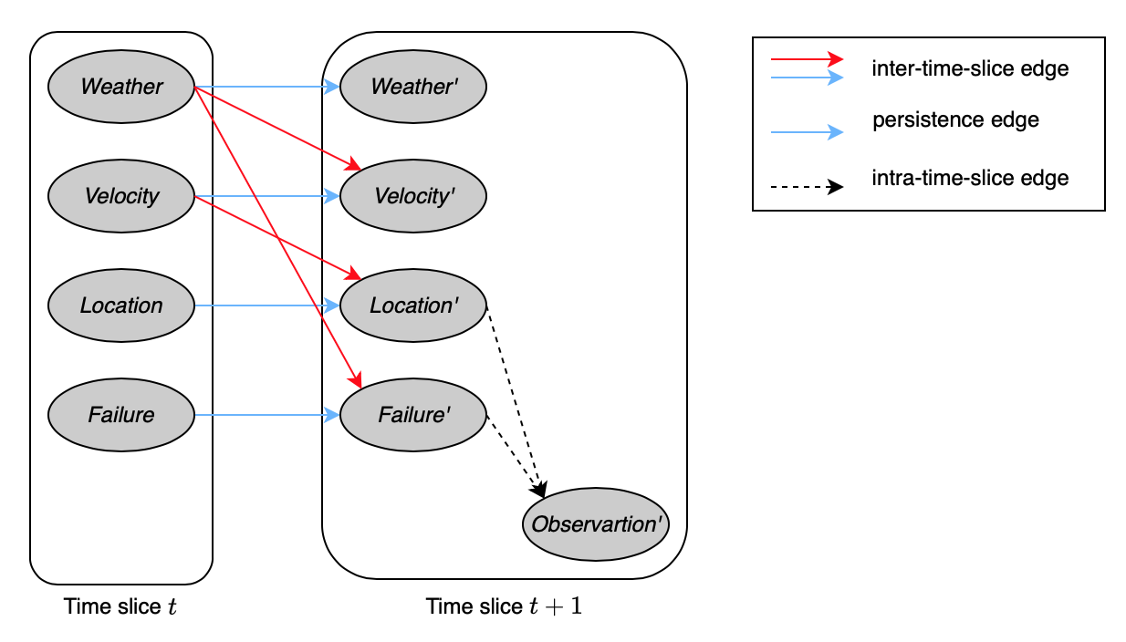
A 2-time-slice Bayesian network (2-TBN) for a process over $\mathcal{X}$ is a conditional Bayesian network over $\mathcal{X}’$ given $\mathcal{X}_I$, where $\mathcal{X}_I\subset\mathcal{X}$ is a set of interface variables.

Hence, as mentioned above, we have

• Only the variables $\mathcal{X}'$ are associated with CPDs (i.e. having parents).
• The interface variables $\mathcal{X}_I$ are variables whose values at time $t$ have a direct effect on the variables at time $t+1$. Thus, only the variables in $\mathcal{X}_I$ can be parents of variables in $\mathcal{X}'$.
• The 2-TBN represents the distribution \begin{equation} P(\mathcal{X}'\vert\mathcal{X})=P(\mathcal{X}'\vert\mathcal{X}_I)=\prod_{i=1}^{n}P(X_i'\vert\text{Pa}_{X_i'}) \end{equation}
• For each template variable $X_i$, the CPD $P(X_i'\vert\text{Pa}_{X_i'})$ is a template factor, i.e. it will be instantiated multiple times within the model, for multiple variables $X_i^{(t)}$ (and their parents).

In a 2-TBN, edges that go between time slices are called inter-time-slice, while the ones connecting variables in the same slices are known as intra-time-slice. Additionally, inter-time-slice edges having the form of $X\rightarrow X’$ are referred as persistence. The variable $X$ for which we have an edge $X\rightarrow X’$ is also called persistent variable.

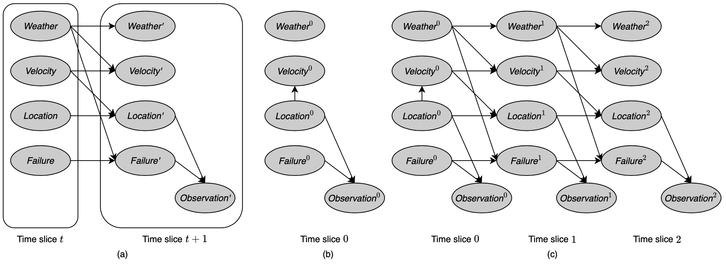
Based on the stationary property, a 2-TBN defines the probability distribution $P(\mathcal{X}^{(t+1)}\vert\mathcal{X}^{(t)})$ for any $t$. Given a distribution over the initial states, we can unroll the network over sequences of any length, to define a Bayesian network that induces a distribution over trajectories of that length.

A dynamic Bayesian network (or DBN) is a tuple $(\mathcal{B}_0,\mathcal{B}_\rightarrow)$, where

• $\mathcal{B}_0$ is a Bayesian network over $\mathcal{X}^{(0)}$ representing the initial distribution over states;
• $\mathcal{B}_\rightarrow$ is a 2-TBN for the process.

For any time span $T\geq0$, the distribution over $\mathcal{X}^{(0:T)}$ is defined as an unrolled Bayesian network, where, for any $i=1,\ldots,n$:

• The structure and CPDs of $X_i^{(0)}$ are the same as those for $X_i$ in $\mathcal{B}_0$.
• The structure and CPDs of $X_i^{(t)}$ for $t>0$ are the same as those for $X_i'$ in $\mathcal{B}_\rightarrow$.

Or in other words, $\mathcal{B}_0$ is the initial state, while $\mathcal{B}_\rightarrow$ represents the transition model.

Remark: Hence, we can view a DBN as a compact representation from which we can generate an infinite set of Bayesian networks (one for every $T>0$).

In DBNs, we can partition the variables $\mathcal{X}$ into disjoint subsets $\mathbf{X}$ and $\mathbf{O}$ such that variables in $\mathbf{X}$ are always hidden, while ones in $\mathbf{O}$ are always observed. This introduces us to an another way of representing temporal process, which is the state-observation model.

State-Observation Models

A state-observation model utilizes two independent assumptions:

• Markov assumption: \begin{equation} (\mathbf{X}^{(t+1)}\perp\mathbf{X}^{(0:t-1)}\vert\mathbf{X}^{(t)}) \end{equation}
• Observations depend on current state only: \begin{equation} (\mathbf{O}^{(t)}\perp\mathbf{X}^{(0:t-1)},\mathbf{X}^{(t+1:\infty)}\vert\mathbf{X}^{(t)}) \end{equation}

Therefore, we can view our probabilistic model containing two components: the transition model, $P(\mathbf{X}’\vert\mathbf{X})$, and the observation model, $P(\mathbf{O}\vert\mathbf{X})$. This corresponds to a 2-TBN structure where the observation variables $\mathbf{O}’$ are all leaves, and have parents only in $\mathbf{X}’$. For instance, as considering Figure 13, $\textit{Observation}’$ are acting as $\mathbf{O}’$.

Hidden Markov Models

A Hidden Markov model, or HMM, is the simplest example of a state-observation model, and also a special case of a simple DBN, which has a sparse transition model $P(S’\vert S)$. Thus, HMMs are often represented using a different graphical notation which visualizes this sparse transition model.

Specifically, in the is representation, the transition model is encoded using a directed graph, where

• Nodes represent the different states of the system, i.e. the values in $\text{Val}(S)$.
• Each directed edge $s\rightarrow s'$ represents a possible transitioning from $s$ to $s'$, i.e. $P(s'\vert s)>0$.

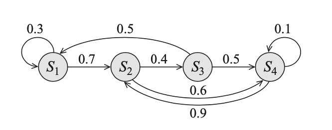
Example 10: Consider an HMM with state variable $S$ that takes 4 possible values $s_1,s_2,s_3,s_4$ and with a transition model

	$s_1$	$s_2$	$s_3$	$s_4$
$s_1$	0.3	0.7	0	0
$s_2$	0	0	0.4	0.6
$s_3$	0.5	0	0	0.5
$s_4$	0	0.9	0	0.1

where the rows correspond to states $s$, while the columns to next states $s’$. On other words, the $i$-th row represents the CPD $P(s’\vert s=s_i)$, and thus must sum to $1$. Its transition graph is shown below

Linear Dynamical Systems

A linear dynamical system, or Kalman filter represents a system of one or more real-valued variable that evolve linearly over time, with some Gaussian noise.

Such systems can be viewed as DBNs where the variables are all continuous and all of the dependencies are linear Gaussian.

They are traditionally represented as a state-observation model, where the state and the observation are both vector-valued r.v.s; and where the transition model and observation model are both encoded using matrices. In more specific, the model is generally defined via the set of equations \begin{align} P(\mathbf{X}^{(t)}\vert\mathbf{X}^{(t-1)})&=\mathcal{N}(A\mathbf{X}^{(t-1)};Q), \\ P(O^{(t)}\vert\mathbf{X}^{(t)})&=\mathcal{N}(H\mathbf{X}^{(t)};R), \end{align} where

• $\mathbf{X}\in\mathbb{R}^n$ is the vector of state variables;
• $O\in\mathbb{R}^m$ is the vector of observation variables;
• $A\in\mathbb{R}^{n\times n}$ (precisely $A\in[0,1]^{n\times n}$) is the transition matrix, defines the linear transition model;
• $H\in\mathbb{R}^{n\times m}$ (also $H\in[0,1]^{n\times m}$ to be exact) defines the linear observation model;
• $R\in\mathbb{R}^{m\times m}$ defines the Gaussian noise associated with the observations.

Extended Kalman Filters

A nonlinear variant of the linear dynamical system, known as extended Kalman filter, is a system where the state transition and observation model are nonlinear functions, i.e. \begin{align} P(\mathbf{X}^{(t)}\vert\mathbf{X}^{(t-1)})&=f(\mathbf{X}^{(t-1)},\mathbf{U}^{(t-1)}) \\ P(O^{(t)}\vert\mathbf{X}^{(t)})&=g(\mathbf{X}^{(t)},\mathbf{W}^{(t)}), \end{align} where

• $f,g$ are nonlinear functions;
• $\mathbf{U}^{(t)},\mathbf{W}^{(t)}$ are Gaussian r.v.s.

Template Variables & Template Factors

As viewing the world as a set of objects, each of which can be divided into a set of mutually exclusive and exhaustive classes $\mathcal{Q}=Q_1,\ldots,Q_k$.

An attribute $A$ is a function $A(U_1,\ldots,U_k)$ whose range is some set $\text{Val}(A)$ and where each argument $U_i$ is known as a logical variable associated with a particular class $Q[U_i]\doteq Q_i$. The tuple $(U_1,\ldots,U_k)$ is called the argument signature of the attribute $A$, denoted $\alpha(A)$ \begin{equation} \alpha(A)\doteq(U_1,\ldots,U_k) \end{equation} Example 11: The argument signature of $\textit{Grade}$ attribute would have two logical variables $S,C$ where $S$ is of class $\textit{Student}$, and where $C$ is of class $\textit{Course}$.

Let $\mathcal{Q}$ be a set of classes, and $\aleph$ be a set of attributes over $\mathcal{Q}$. An object skeleton $\kappa$ specifies a fixed, finite set of objects $\mathcal{O}^\kappa[Q]$ for every $Q\in\mathcal{Q}$. We also define \begin{equation} \mathcal{O}^\kappa[\alpha(A)]=\mathcal{O}^\kappa[U_1,\ldots,U_k]\doteq\mathcal{O}^\kappa[Q[U_1]]\times\ldots\times\mathcal{O}^\kappa[Q[U_k]] \end{equation} By default, we let $\Gamma_\kappa[A]=\mathcal{O}^\kappa[\alpha(A)]$ to be the set of possible assignments to the logical variables in the argument signature of $A$. However, an object skeleton might also specify a subset of legal assignments, i.e. $\Gamma_\kappa[A]\subset\mathcal{O}^\kappa[\alpha(A)]$.

For an object skeleton $\kappa$ over $\mathcal{Q},\aleph$. We define sets of ground random variables \begin{align} \mathcal{X}_\kappa[A]&\doteq\{A(\gamma):\gamma\in\Gamma_\kappa[A]\} \\ \mathcal{X}_\kappa[\aleph]&\doteq\bigcup_{A\in\aleph}\mathcal{X}_\kappa[A] \end{align} Here, we are abusing notation, identifying an argument $\gamma=(U_1\mapsto u_1,\ldots,U_k\mapsto u_k)$ with the tuple $(u_1,\ldots,u_k)$.

A template factor $\xi$ is a function defined over a tuple of template attributes $A_1,\ldots,A_l$ where each $A_i$ has a range $\text{Val}(A_i)$. It defines a mapping $\text{Val}(A_1)\times\ldots\times\text{Val}(A_l)\mapsto\mathbb{R}$. Given r.v.s $X_1,\ldots,X_l$ such that $\text{Val}(X_i)=\text{Val}(A_i)$ for all $i=1,\ldots,j$, we define $\xi(X_1,\ldots,X_l)$ to be the instantiated factor from $\mathbf{X}$ to $\mathbb{R}$.

Directed Probabilistic Models for Object-Relational

Plate Models

A plate model $\mathcal{M}_\text{Plate}$ defines for each template attribute $A\in\aleph$ with argument signature $U_1,\ldots,U_k$:

• a set of template parents \begin{equation} \text{Pa}_A=\{B_1(\mathbf{U}_1),\ldots,B_l(\mathbf{U}_l)\}, \end{equation} such that for each $B_i(\mathbf{U}_i)$, we have that $\mathbf{U}_i\subset\{U_1,\ldots,U_k\}$. The variables $\mathbf{U}_i$ are the argument signature of the parent $B_i$.
• a template CPD $P(A\vert\text{Pa}_A)$.

Ground Bayesian Networks for Plate Models

A plate model $\mathcal{M}_\text{Plate}$ and object skeleton $\kappa$ define a ground Bayesian network $\mathcal{B}_\kappa^{\mathcal{M}_\text{Plate}}$ as follows. Let $A(U_1,\ldots,U_k)$ be any template attribute in $\aleph$. Then, for any $\gamma=(U_1\mapsto u_1,\ldots,U_k\mapsto u_k)\in\Gamma_\kappa[A]$, we have a variable $A(\gamma)$ in the ground network, with parents $B(\gamma)$ for all $B\in\text{Pa}_A$, and the instantiated CPD $P(A(\gamma)\vert\text{Pa}_A(\gamma))$.

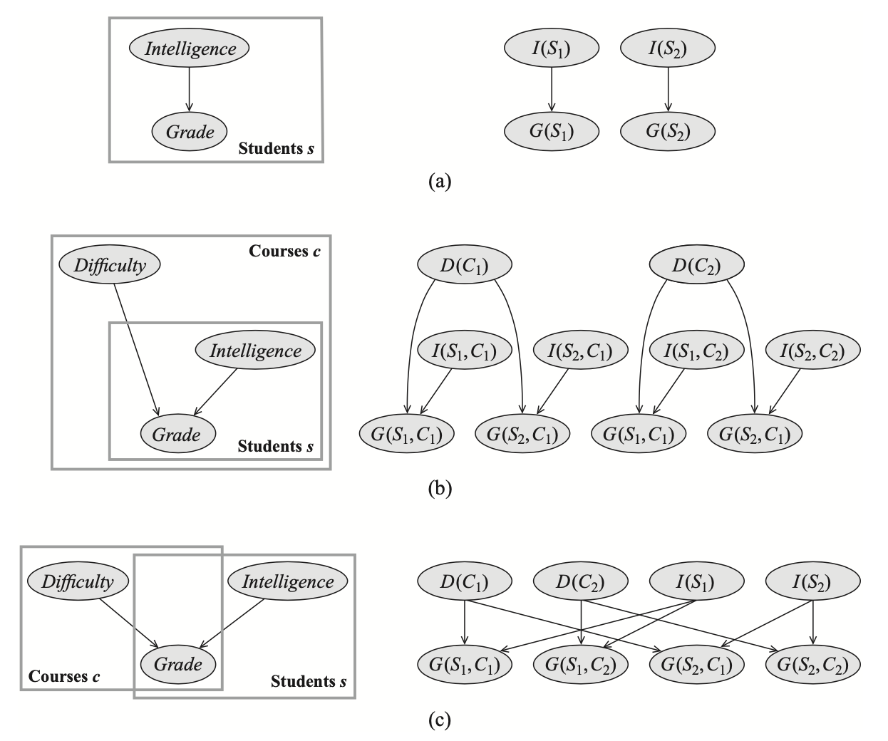
Example 12: Consider the Figure 15(c), without loss of generality, we have that:

• The plate model $\mathcal{M}_\text{Plate}$ is defined over a set $\aleph=\{\textit{Grade},\textit{Difficulty},\textit{Intelligence}\}$ of template attributes, for each of which:
  • $\alpha(\textit{Grade})=(S,C)$ and $\text{Pa}_\textit{Grade}=\{\textit{Difficulty}(C),\textit{Intelligence}(S)\}$;
  • $\alpha(\textit{Difficulty})=(C)$ and $\text{Pa}_\textit{Difficulty}=\emptyset$;
  • $\alpha(\textit{Intelligence})=(S)$ and $\text{Pa}_\textit{Intelligence}=\emptyset$,
  where $S$ is logical variable of class $\textit{Student}$, and $C$ is a logical variable of class $\textit{Course}$.
• Let $(S\mapsto s,C\mapsto c)$ be some assignment to some logical variables $S,C$ where $S$ is of class $\textit{Student}$, $C$ is of class $\textit{Course}$. We then have instantiated CPDs: \begin{align} P(G(s,c)\vert\text{Pa}_G(s,c))&=P(G(s,c)\vert D(s,c),I(s,c))=P(G(s,c)\vert D(c),I(s)), \\ P(D(c)\vert\text{Pa}_D(c))&=P(D(c)), \\ P(I(s)\vert\text{Pa}_I(s))&=P(I(s)) \end{align}

Probabilistic Relational Models

For a template attribute $A$, we define a contingent dependency model as a tuple containing:

• A parent argument signature $\alpha(\text{Pa}_A)$, which is a tuple of typed logical variables $U_i$ such that $\alpha(\text{Pa}_A)\supset\alpha(A)$.
• A guard $\Gamma$, which is a binary-valued formula defined in terms of a set of template attributes $\text{Pa}_A^\Gamma$ over the argument signature $\alpha(\text{Pa}_A)$.
• A set of template parents \begin{equation} \text{Pa}_A=\{B_1(\mathbf{U}_1),\ldots,B_l(\mathbf{U}_l)\}, \end{equation} such that for each $B_i(\mathbf{U}_i)$, we have that $\mathbf{U}_i\subset\alpha(\text{Pa}_A)$.

A probabilistic relational model (or PRM) $\mathcal{M}_\text{PRM}$ defines, for each $A\in\aleph$ a contingent dependency model and a template CPD.

Ground Bayesian Networks for PRMs

A PRM $\mathcal{M}_\text{PRM}$ and object skeleton $\kappa$ define a ground Bayesian network $\mathcal{B}_\kappa^{\mathcal{M}_\text{PRM}}$ as follows. Let $A(U_1,\ldots,U_k)$ be any template attribute in $\aleph$. Then, for any assignment $\gamma\in\Gamma_\kappa[A]$, we have a variable $A(\gamma)$ in the ground network. This variable has, for any $B\in\text{Pa}_A^\Gamma\cup\text{Pa}_A$ and any assignment $\gamma’$ to $\alpha(\text{Pa}_A)\backslash\alpha(A)$, the parent that is the instantiated variable $B(\gamma,\gamma’)$.

Undirected Representation

A relational Markov network $\mathcal{M}_\text{RMN}$ is defined in terms of a set $\Lambda$ of template features, where each $\lambda\in\Lambda$ contains:

• a real-valued template feature $f_\lambda$ whose arguments are $\aleph(\lambda)=\{A_1(\mathbf{U}_1),\ldots,A_l(\mathbf{U}_l)\}$;
• a weight $w_\lambda\in\mathbb{R}$.

Ground Gibbs Distribution

Given an RMN $\mathcal{M}_\text{RMN}$, an object skeleton $\kappa$, we can define a ground Gibbs distribution $P_\kappa^{\mathcal{M}_\text{RMN}}$ as:

• The variables in the network are $\mathcal{X}_\kappa[\aleph]$ (as defined above);
• $P_\kappa^{\mathcal{M}_\text{RMN}}$ contains a term \begin{equation} \exp\big(w_\lambda f_\lambda(\gamma)\big), \end{equation} for each feature template $\lambda\in\Lambda$ and each assignment $\gamma\in\Gamma_\kappa[\alpha(\lambda)]$.

References

[1] Daphne Koller, Nir Friedman. Probabilistic Graphical Models. The MIT Press.

[2] Michael I. Jordan. An Introduction to Probabilistic Graphical Models. In preparation.

[3] Eric P. Xing. 10-708: Probabilistic Graphical Model. CMU Spring 2020.

[4] Stefano Ermon. CS228: Probabilistic Graphical Model. Stanford Winter 2017-2018.

Footnotes