Notes on Learning in PGMs.
Parameter Learning
Fully Observed Data
MLE for Bayesian Networks
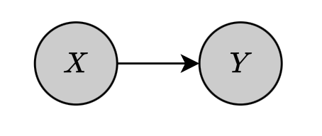
Suppose that we have a Bayesian network of two binary nodes $X,Y$ connected by $X\to Y$.
The network is parameterized by a parameter vector $\boldsymbol{\theta}$, which defines the set of parameters of all the CPDs in the network, i.e. \begin{equation} \boldsymbol{\theta}_X=\{\theta_{x^0},\theta_{x^1}\} \end{equation} and \begin{equation} \boldsymbol{\theta}_{Y\vert X}=\boldsymbol{\theta}_{Y\vert x_0}\cup\boldsymbol{\theta}_{Y\vert x^1}=\{\theta_{y^0\vert x^0},\theta_{y^1\vert x^0}\}\cup\{\theta_{y^0\vert x^1},\theta_{y^1\vert x^1}\} \end{equation} Assuming that we are given the training set \begin{equation} \mathcal{D}=\{(x[1],y[1]),\ldots,(x[M],y[M])\} \end{equation} which describes $M$ instances of variables $X$ and $Y$. The likelihood function is then given as \begin{align} L(\boldsymbol{\theta}:\mathcal{D})&=\prod_{m=1}^{M}P(x[m],y[m];\boldsymbol{\theta}) \\ &=\prod_{m=1}^{M}P(x[m];\boldsymbol{\theta})P(y[m]\big\vert x[m];\boldsymbol{\theta}) \\ &=\left(\prod_{m=1}^{M}P(x[m];\boldsymbol{\theta})\right)\left(\prod_{m=1}^{M}P(y[m]\big\vert x[m];\boldsymbol{\theta})\right), \end{align} which decomposes into two terms, on for each variable. Each of these are referred as local likelihood function that measures how well the variable is predicted given its parents.
Global Likelihood Decomposition
Generally, suppose that we want to learn a parameters $\boldsymbol{\theta}$ for Bayesian network structure $\mathcal{G}$. Given a dataset $\mathcal{D}=\{\xi[1],\ldots,\xi[M]\}$, analogy to the argument above, we have that the likelihood function is given by \begin{align} L(\boldsymbol{\theta}:\mathcal{D})&=\prod_{m=1}^{M}P_\mathcal{G}(\xi[m];\boldsymbol{\theta}) \\ &=\prod_{m=1}^{M}\prod_i P\big(x_i[m]\big\vert\text{pa}_{X_i}[m];\boldsymbol{\theta}\big) \\ &=\prod_i\left[\prod_{m=1}^{M}P\big(x_i[m]\big\vert\text{pa}_{X_i}[m];\boldsymbol{\theta}\big)\right]\label{eq:gld.1} \end{align} Each of the terms in the square brackets refers to the conditional likelihood of a particular variable given its parents in the network. Also, let $\boldsymbol{\theta}_{X_i\vert\text{Pa}_{X_i}}$ denote the subset of parameters that determines $P(X_i\vert\text{Pa}_{X_i})$. Thus, the local likelihood function for $X_i$ is then given by \begin{equation} L_i(\boldsymbol{\theta}_{X_i\vert\text{Pa}_{X_i}}:\mathcal{D})=\prod_{m=1}^{M}P\big(x_i[m]\big\vert\text{pa}_{X_i}[m];\boldsymbol{\theta}_{X_i\vert\text{Pa}_{X_i}}\big), \end{equation} which allows us to rewrite the likelihood function \eqref{eq:gld.1} as \begin{equation} L(\boldsymbol{\theta}:\mathcal{D})=\prod_i L_i(\boldsymbol{\theta}_{X_i\vert\text{Pa}_{X_i}}:\mathcal{D}) \end{equation} In other words, when $\boldsymbol{\theta}_{X_i\vert\text{Pa}_{X_i}}$ are disjoint, the likelihood can be decomposed as a product of independent terms, one for each CPD of the network. This property is known as the global decomposition of the likelihood function.
Additionally, we can maximize each local likelihood function $L_i(\boldsymbol{\theta}_{X_i\vert\text{Pa}_{X_i}}:\mathcal{D})$ independently of the others, and then combine the solutions together to get an MLE solution.
Table-CPDs
As the MLE solution for a Bayesian network can be computed via parameterization of its CPDs, we now consider the simplest parameterization of the CPD, tabular CPD, or table-CPD.
Suppose we have a variable $X$ with parents $\mathbf{U}$. If we represent the CPD $P(X\vert\mathbf{U})$ as a table, we then have a parameter $\theta_{x\vert\mathbf{u}}$ for each $x\in\text{Val}(X)$ and $\mathbf{u}\in\text{Val}(\mathbf{U})$. The local likelihood function is then can be decomposed further as \begin{align} L_X(\boldsymbol{\theta}_{X\vert\mathbf{U}})&=\prod_{m=1}^{M}\theta_{x[m]\vert\mathbf{u}[m]} \\ &=\prod_{\mathbf{u}\in\text{Val}(\mathbf{U})}\left(\prod_{x\in\text{Val}(X)}\theta_{x\vert\mathbf{u}}^{M[\mathbf{u},x]}\right), \end{align} where $M[\mathbf{u},x]$ is the number of times $x[m]=x$ and $\mathbf{u}[m]=\mathbf{u}$ in $\mathcal{D}$.
Gaussian Bayesian Networks
Consider a variable $X$ with parents $\mathbf{U}=\{U_1,\ldots,U_k\}$ with a linear Gaussian CPD \begin{equation} P(X\vert\mathbf{u})=\mathcal{N}(\beta_0+\beta_1 u_1+\ldots+\beta_k u_k;\sigma^2) \end{equation} Thus, we have that \begin{equation} P(x\vert\mathbf{u})=\frac{1}{\sqrt{2\pi}\sigma}\exp\left[-\frac{(\beta_0+\beta_1 u_1+\ldots+\beta_k u_k-x)^2}{2\sigma^2}\right] \end{equation} Our task is to learn the parameters $\boldsymbol{\theta}_{X\vert\mathbf{U}}=(\beta_0,\ldots,\beta_k,\sigma)$. We continue by considering the log-likelihood \begin{align} \ell_X(\boldsymbol{\theta}_{X\vert\mathbf{U}}:\mathcal{D})&=\log L_X(\boldsymbol{\theta}_{X\vert\mathbf{U}}) \\ &=\log\prod_{m=1}^{M}P\big(x[m]\big\vert\mathbf{u}[m];\boldsymbol{\theta}_{X\vert\mathbf{U}}\big) \\ &=\sum_{m=1}^{M}\log P\big(x[m]\big\vert\mathbf{u}[m];\boldsymbol{\theta}_{X\vert\mathbf{U}}\big) \\ &=\sum_{m=1}^{M}\left[\frac{1}{2}\log(2\pi\sigma^2)-\frac{1}{2}\frac{1}{\sigma^2}\big(\beta_0+\beta_1 u_1[m]+\ldots+\beta_k u_k[m]-x[m]\big)^2\right] \end{align} Taking the derivative of the log-likelihood w.r.t $\beta_0$ gives us \begin{align} \frac{\partial}{\partial\beta_0}\ell_X(\boldsymbol{\theta}_{X\vert\mathbf{U}}:\mathcal{D})&=\sum_{m=1}^{M}-\frac{1}{\sigma^2}\big(\beta_0+\beta_1 u_1[m]+\ldots+\beta_k u_k[m]-x[m]\big) \\ &=-\frac{1}{\sigma^2}\left(M\beta_0+\beta_1\sum_{m=1}^{M}u_1[m]+\ldots+\beta_k\sum_{m=1}^{M}u_k[m]-\sum_{m=1}^{M}x[m]\right) \end{align} Setting the derivative to zero, we have that \begin{equation} \frac{1}{M}\sum_{m=1}^{M}x[m]=\beta_0+\beta_1\frac{1}{M}\sum_{m=1}^{M}u_1[m]+\ldots+\beta_k\frac{1}{M}\sum_{m=1}^{M}u_k[m]\label{eq:gbn.1} \end{equation} Then, if we define \begin{equation} \mathbb{E}_\mathcal{D}[X]\doteq\frac{1}{M}\sum_{m=1}^{M}x[m], \end{equation} which represents the average value a variable $X$. Thus, we can rewrite \eqref{eq:gbn.1} as \begin{equation} \mathbb{E}_\mathcal{D}[X]=\beta_0+\beta_1\mathbb{E}_\mathcal{D}[U_1]+\ldots+\beta_k\mathbb{E}_\mathcal{D}[U_k]\label{eq:gbn.2} \end{equation} On the other hand, differentiating the log-likelihood function w.r.t $\beta_i$ for $i\neq 0$ gives us \begin{align} &\hspace{-0.5cm}\frac{\partial}{\partial\beta_i}\ell_X(\boldsymbol{\theta}_{X\vert\mathbf{U}}:\mathcal{D})\nonumber \\ &\hspace{-0.5cm}=\sum_{m=1}^{M}-\frac{u_i[m]}{\sigma^2}\big(\beta_0+\beta_1 u_1[m]+\ldots+\beta_k u_k[m]-x[m]\big) \\ &\hspace{-0.5cm}=-\frac{1}{\sigma^2}\left(M\beta_0+\beta_1\sum_{m=1}^{M}u_1[m]u_i[m]+\ldots+\beta_k\sum_{m=1}^{M}u_k[m]u_i[m]-\sum_{m=1}^{M}x[m]u_i[m]\right) \end{align} Similarly, setting this derivative to zero lets us obtain \begin{equation} \mathbb{E}_\mathcal{D}[X U_i]=\beta_0\mathbb{E}_\mathcal{D}[U_i]+\beta_1\mathbb{E}_\mathcal{D}[U_1 U_i]+\ldots+\beta_k\mathbb{E}_\mathcal{D}[U_k U_i]\label{eq:gbn.3} \end{equation} From the results \eqref{eq:gbn.2} and \eqref{eq:gbn.3}, we can find the MLE solution $\hat{\boldsymbol{\beta}}$ by solving the system of linear equations \begin{equation} \left[\begin{matrix}1&\mathbb{E}_\mathcal{D}[U_1]&\ldots&\mathbb{E}_\mathcal{D}[U_k] \\ \mathbb{E}_\mathcal{D}[U_1]&\mathbb{E}_\mathcal{D}[U_1 U_1]&\ldots&\mathbb{E}_\mathcal{D}[U_1 U_k] \\ \vdots&\vdots&\ddots&\vdots \\ \mathbb{E}_\mathcal{D}[U_k]&\mathbb{E}_\mathcal{D}[U_k U_1]&\ldots&\mathbb{E}_\mathcal{D}[U_k U_k]\end{matrix}\right]\left[\begin{matrix}\beta_0 \\ \beta_1 \\ \vdots \\ \beta_k\end{matrix}\right]=\left[\begin{matrix}\mathbb{E}_\mathcal{D}[X] \\ \mathbb{E}_\mathcal{D}[X U_1] \\ \vdots \\ \mathbb{E}_\mathcal{D}[X U_k]\end{matrix}\right] \end{equation} Additionally, by multiplying both sides of \eqref{eq:gbn.2} with $\mathbb{E}_\mathcal{D}[U_i]$, we have \begin{equation} \mathbb{E}_\mathcal{D}[X]\mathbb{E}_\mathcal{D}[U_i]=\beta_0\mathbb{E}_\mathcal{D}[U_i]+\beta_1\mathbb{E}_\mathcal{D}[U_1]\mathbb{E}_\mathcal{D}[U_i]+\ldots+\beta_k\mathbb{E}_\mathcal{D}[U_k]\mathbb{E}_\mathcal{D}[U_i] \end{equation} Then, subtracting this equation from \eqref{eq:gbn.3} gives us \begin{align} \mathbb{E}_\mathcal{D}[X U_i]-\mathbb{E}_\mathcal{D}[X]\mathbb{E}_\mathcal{D}[U_i]&=\beta_1\big(\mathbb{E}_\mathcal{D}[U_1 U_i]-\mathbb{E}_\mathcal{D}[U_1]\mathbb{E}_\mathcal{D}[U_i]\big)+\ldots+\nonumber \\ &\hspace{0.6cm}\beta_k\big(\mathbb{E}_\mathcal{D}[U_k U_i]-\mathbb{E}_\mathcal{D}[U_k]\mathbb{E}_\mathcal{D}[U_i]\big), \end{align} or \begin{equation} \text{Cov}_\mathcal{D}[X,U_i]=\beta_1\text{Cov}_\mathcal{D}[U_1,U_i]+\ldots+\beta_k\text{Cov}_\mathcal{D}[U_k,U_i]\label{eq:gbn.4} \end{equation} where we have defined $\text{Cov}_\mathcal{D}[X,U_i]$ as the observed covariance of $X$ and $U_i$ in the data.
Finally, differentiating the log-likelihood w.r.t $\sigma^2$, we have that \begin{equation} \frac{\partial}{\partial\sigma}\ell_X(\boldsymbol{\theta}_{X\vert\mathbf{U}}:\mathcal{D})=\sum_{m=1}^{M}\left[\frac{1}{2}\frac{1}{\sigma^2}+\frac{1}{2}\frac{1}{(\sigma^2)^2}\big(\beta_0+\beta_1 u_1[m]+\ldots+\beta_k u_k[m]-x[m]\big)^2\right] \end{equation} Analogously, setting this derivative to zero, we have that \begin{equation} \sigma^2=\text{Cov}_\mathcal{D}[X,X]-\sum_{i=1}^{k}\sum_{j=1}^{k}\beta_i\beta_j\text{Cov}_\mathcal{D}[U_i,U_j]\label{eq:gbn.5} \end{equation}
Remark
Example 1: Let us estimate a joint multivariate Gaussian distribution. Specifically, consider continuous r.v.s $X$ and $Y$ and assume we have a dataset of $M$ samples $\mathcal{D}=\{(x[1],y[1]),\ldots,(x[M],y[M])\}$. Our job is to find the MLE estimate for a joint Gaussian distribution over $X,Y$.
Let $\mathbf{Z}$ be a random vector that encodes the joint distribution of $X$ and $Y$. In particular \begin{equation} \mathbf{Z}=\left[\begin{matrix}X \\ Y\end{matrix}\right] \end{equation} We have that $\mathbf{Z}\sim\mathcal{N}(\boldsymbol{\mu},\boldsymbol{\Sigma})$ with \begin{equation} \boldsymbol{\mu}=\left[\begin{matrix}\mu_X \\ \mu_Y\end{matrix}\right],\hspace{1cm}\boldsymbol{\Sigma}=\left[\begin{matrix}\Sigma_{XX}&\Sigma_{XY} \\ \Sigma_{YX}&\Sigma_{YY}\end{matrix}\right] \end{equation} Thus, we have that \begin{equation} P(\mathbf{z})=\frac{1}{2\pi\vert\boldsymbol{\Sigma}\vert^{1/2}}\exp\left[-\frac{1}{2}(\mathbf{z}-\boldsymbol{\mu})^\text{T}\boldsymbol{\Sigma}^{-1}(\mathbf{z}-\boldsymbol{\mu})\right] \end{equation} Our job then is to learn the parameter $\boldsymbol{\theta}=(\boldsymbol{\mu},\boldsymbol{\Sigma})$. We begin by considering the log-likelihood function \begin{align} \ell(\boldsymbol{\theta})&=\log\prod_{m=1}^{M}P(x[m],y[m];\boldsymbol{\theta}) \\ &=\log\prod_{m=1}^{M}\frac{1}{2\pi\vert\boldsymbol{\Sigma}\vert^{1/2}}\exp\left[-\frac{1}{2}(\mathbf{z}[m]-\boldsymbol{\mu})^\text{T}\boldsymbol{\Sigma}^{-1}(\mathbf{z}[m]-\boldsymbol{\mu})\right] \\ &=\sum_{m=1}^{M}-\log(2\pi)-\frac{1}{2}\log\vert\boldsymbol{\Sigma}\vert-\frac{1}{2}(\mathbf{z}[m]-\boldsymbol{\mu})^\text{T}\boldsymbol{\Sigma}^{-1}(\mathbf{z}[m]-\boldsymbol{\mu}) \end{align} Taking the derivative of the log-likelihood w.r.t $\boldsymbol{\mu}$ gives us \begin{align} \frac{\partial}{\partial\boldsymbol{\mu}}\ell(\boldsymbol{\theta})&=\sum_{m=1}^{M}\frac{1}{2}\big[\boldsymbol{\Sigma}^{-1}(\mathbf{z}[m]-\boldsymbol{\mu})-(\boldsymbol{\Sigma}^{-1})^\text{T}(\mathbf{z}[m]-\boldsymbol{\mu})\big] \\ &=\sum_{m=1}^{M}\boldsymbol{\Sigma}^{-1}(\mathbf{z}[m]-\boldsymbol{\mu}), \end{align} where we have used the fact that the covariance matrix $\boldsymbol{\Sigma}$ is symmetric. Setting the derivative to zero we obtain the MLE solution for $\boldsymbol{\mu}$ \begin{equation} \boldsymbol{\mu}=\frac{1}{M}\sum_{m=1}^{M}\mathbf{z}[m]=\left[\begin{matrix}\mathbb{E}_\mathcal{D}[X] \\ \mathbb{E}_\mathcal{D}[Y]\end{matrix}\right] \end{equation} On the other hand, differentiating the log-likelihood w.r.t $\boldsymbol{\Sigma}$, we obtain \begin{align} \frac{\partial}{\partial\boldsymbol{\Sigma}}\ell(\boldsymbol{\theta})&=\sum_{m=1}^{M}-\frac{1}{2}\frac{\vert\boldsymbol{\Sigma}\vert\boldsymbol{\Sigma}^{-1}}{\vert\boldsymbol{\Sigma}\vert}+\frac{1}{2}\big[(\boldsymbol{\Sigma}^{-1})^\text{T}(\mathbf{z}[m]-\boldsymbol{\mu})(\mathbf{z}[m]-\boldsymbol{\mu})^\text{T}(\boldsymbol{\Sigma}^{-1})^\text{T}\big] \\ &=\frac{1}{2}\sum_{m=1}^{M}\boldsymbol{\Sigma}^{-1}(\mathbf{z}[m]-\boldsymbol{\mu})(\mathbf{z}[m]-\boldsymbol{\mu})^\text{T}\boldsymbol{\Sigma}^{-1}-\boldsymbol{\Sigma}^{-1} \end{align} Setting this derivative to zero, we have that \begin{align} \boldsymbol{\Sigma}&=\sum_{m=1}^{M}(\mathbf{z}[m]-\boldsymbol{\mu})(\mathbf{z}[m]-\boldsymbol{\mu})^\text{T} \\ &=\sum_{m=1}^{M}\left[\begin{matrix}(x[m]-\mu_X)^2&(x[m]-\mu_X)(y[m]-\mu_Y) \\ (y[m]-\mu_Y)(x[m]-\mu_X)&(y[m]-\mu_Y)^2\end{matrix}\right] \\ &=\left[\begin{matrix}\text{Cov}_\mathcal{D}[X,X]&\text{Cov}_\mathcal{D}[X,Y] \\ \text{Cov}_\mathcal{D}[Y,X]&\text{Cov}_\mathcal{D}[Y,Y]\end{matrix}\right] \end{align}
Bayesian Parameter Estimation
General setting
In the Bayesian approach, as before, we assume a general learning problem where we observe a training set $\mathcal{D}=\{\xi[1],\ldots,\xi[M]\}$ and a parametric model $P(\xi\vert\boldsymbol{\theta})$ where we can choose parameters from a parameter space $\Theta$, i.e. in this case, samples according to the probabilistic model are conditionally i.i.d given $\boldsymbol{\theta}$ instead of, recalling that in MLE, being (unconditionally) i.i.d.
Priors, Posteriors
To perform the task, we need to define a joint distribution $P(\mathcal{D},\boldsymbol{\theta})$ over the data and the parameters, which can be written by \begin{equation} P(\mathcal{D},\boldsymbol{\theta})=P(\mathcal{D}\vert\boldsymbol{\theta})P(\boldsymbol{\theta}), \end{equation} where
- $P(\mathcal{D}\vert\boldsymbol{\theta})$ is the likelihood function, which is the probability of the observations given the parameters, as in the MLE approach.
- $P(\boldsymbol{\theta})$ is referred as the prior distribution, which encodes our prior beliefs, i.e. before data is observed.
By Bayes’ rule, from the likelihood and prior, combined with the defined joint distribution, we can derive the so-called posterior distribution over the parameters, which corresponds to our beliefs after observing the data, as \begin{align} P(\boldsymbol{\theta}\vert\mathcal{D})&=\frac{P(\mathcal{D}\vert\boldsymbol{\theta})P(\boldsymbol{\theta})}{P(\mathcal{D})} \\ &=\frac{P(\mathcal{D}\vert\boldsymbol{\theta})P(\boldsymbol{\theta})}{\int_\Theta P(\mathcal{D}\vert\boldsymbol{\theta}’)P(\boldsymbol{\theta}’)d\boldsymbol{\theta}’}, \end{align} where, since the denominator is just a normalizing constant, can be expressed as \begin{equation} P(\boldsymbol{\theta}\vert\mathcal{D})\propto P(\mathcal{D}\vert\boldsymbol{\theta})P(\boldsymbol{\theta}) \end{equation} Since the posterior is a (normalized) product of the prior and the likelihood, it seems natural to require that the prior also have a form similar to the likelihood, such priors are referred as conjugate priors.
More formally, a family of priors $P(\boldsymbol{\theta}:\boldsymbol{\alpha})$ is conjugate to a particular model $P(\xi\vert\boldsymbol{\theta})$ if for any possible dataset $\mathcal{D}$ of i.i.d samples from $P(\xi\vert\boldsymbol{\theta})$, and any choice of legal hyperparameters $\boldsymbol{\alpha}$ for the prior over $\boldsymbol{\theta}$, there are hyperparameters $\boldsymbol{\alpha}’$ that describe the posterior, i.e. \begin{equation} P(\boldsymbol{\theta}:\boldsymbol{\alpha}’)\propto P(\mathcal{D}\vert\boldsymbol{\theta})P(\boldsymbol{\theta}:\boldsymbol{\alpha}) \end{equation}
Example 2: If we select Dirichlet as the prior distribution, specifically, let $\boldsymbol{\theta}=(\theta_1,\ldots,\theta_K)$ and $\boldsymbol{\theta}\sim\text{Dirichlet}(\alpha_1,\ldots,\alpha_K)$, we have that \begin{equation} P(\boldsymbol{\theta})\propto\prod_{k=1}^{K}\theta_k^{\alpha_k-1} \end{equation} Then we have that the posterior $P(\boldsymbol{\theta}\vert\mathcal{D})$ is $\text{Dirichlet}(\alpha_1+M[1],\ldots,\alpha_K+M[K])$, where $M[k]$ is the number of occurrences of $x^k$.
Bayesian Estimator
From the posterior, we can predict the probability of future samples. Specifically, suppose that we are about to sample a new instance $\xi[M+1]$, then the Bayesian estimator, or the predictive distribution, is the posterior distribution over a new example. \begin{align} P(\xi[M+1]\vert\mathcal{D})&=\int P(\xi[M+1]\vert\mathcal{D},\boldsymbol{\theta})P(\boldsymbol{\theta}\vert\mathcal{D})d\boldsymbol{\theta} \\ &=\int P(\xi[M+1]\vert\boldsymbol{\theta})P(\boldsymbol{\theta}\vert\mathcal{D})d\boldsymbol{\theta} \\ &=\mathbb{E}_{P(\boldsymbol{\theta}\vert\mathcal{D})}\big[P(\xi[M+1]\vert\boldsymbol{\theta})\big], \end{align} where in the second step, we use the fact that samples are i.i.d given $\boldsymbol{\theta}$.
Bayesian Parameter Estimation in Bayesian Networks
Since in Bayesian framework, it is required to specify a joint distribution over the training examples and the unknown parameters. Additionally, this joint distribution can be considered as a Bayesian network.
Parameter Independence and Global Decomposition
Suppose that we want to estimate parameters for a networks consisting of two variables $X$ and $Y$ with edge $X\rightarrow Y$. Also, we are given a training dataset $\mathcal{D}=\{(x[1],y[1]),\ldots,(x[M],y[M])\}$. Additionally, we have unknown parameters $\boldsymbol{\theta}_X,\boldsymbol{\theta}_{Y\vert X}$. The dependencies between variables are described in the following network.
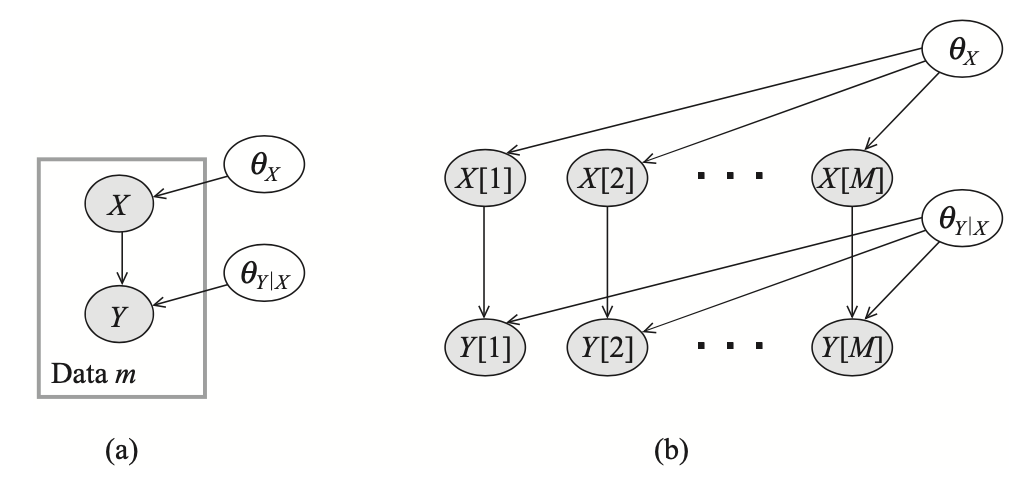
We have already known that in using Bayesian approach, the samples are independent given the parameters, i.e. \begin{equation} \text{d-sep}(\{X[m],Y[m]\};\{X[m’],Y[m’]\}\vert\{\boldsymbol{\theta}_X,\boldsymbol{\theta}_{Y\vert X}\}), \end{equation} which can be justified by an examination of active trails from the above figure. Moreover, the network structure given in Figure 1 also satisfies the global parameter independence.
Let $\mathcal{G}$ be a BN structure with parameters $\boldsymbol{\theta}=(\boldsymbol{\theta}_{X_1\vert\text{Pa}_{X_1}},\ldots,\boldsymbol{\theta}_{X_n\vert\text{Pa}_{X_n}})$. Then, a prior $P(\boldsymbol{\theta})$ is said to satisfy global parameter independence if it has the form \begin{equation} P(\boldsymbol{\theta})=\prod_{i=1}^{n}P(\boldsymbol{\theta}_{X_i\vert\text{Pa}_{X_i}}) \end{equation} This property allows us to conclude that complete data, $\mathcal{D}$, d-separates the parameters for different CPDs, i.e. \begin{equation} \text{d-sep}\big(\boldsymbol{\theta}_X;\boldsymbol{\theta}_{Y\vert X}\big\vert\mathcal{D}\big) \end{equation} This is due to for each $m$, we have that any path between $X[m]$ and $Y[m]$ has the form \begin{equation} \boldsymbol{\theta}_X\rightarrow X[m]\rightarrow Y[m]\leftarrow\boldsymbol{\theta}_{Y\vert X}, \end{equation} which is inactive given the observation $x[m],y[m]$. Thus, we obtain that \begin{equation} P(\boldsymbol{\theta}_X,\boldsymbol{\theta}_{Y\vert X}\vert\mathcal{D})=P(\boldsymbol{\theta}_X\vert\mathcal{D})P(\boldsymbol{\theta}_{Y\vert X}\vert\mathcal{D}) \end{equation} This decomposition suggests that given $\mathcal{D}$, we can find the solution for the posterior over $\boldsymbol{\theta}$ by independently finding the result corresponding to the posterior over each of $\boldsymbol{\theta}_X$ and $\boldsymbol{\theta}_{Y\vert X}$, which is analogous to the global likelihood decomposition in the MLE. In Bayesian setting this property has additional importance.
Generally, suppose that we are given a Bayesian network graph $\mathcal{G}$ with parameters $\boldsymbol{\theta}$. As mentioned before that in using Bayesian approach, we need to specify a prior distribution over the parameter space $P(\boldsymbol{\theta})$ and a posterior distribution over the parameters given the samples $\mathcal{D}$ \begin{equation} P(\boldsymbol{\theta}\vert\mathcal{D})=\frac{P(\mathcal{D}\vert\boldsymbol{\theta})P(\boldsymbol{\theta})}{P(\mathcal{D})}\label{eq:pigd.1} \end{equation} Moreover, assuming that we have global parameter independence, then combining with the global likelihood decomposition mentioned above, the posterior in \eqref{eq:pigd.1} can be continued to derive as a product of local terms: \begin{align} P(\boldsymbol{\theta}\vert\mathcal{D})&=\frac{P(\mathcal{D}\vert\boldsymbol{\theta})P(\boldsymbol{\theta})}{P(\mathcal{D})} \\ &=\frac{1}{P(\mathcal{D})}\left(\prod_i L_i(\boldsymbol{\theta}_{X_i\vert\text{Pa}_{X_i}}:\mathcal{D})\right)\left(\prod_i P(\boldsymbol{\theta}_{X_i\vert\text{Pa}_{X_i}})\right) \\ &=\frac{1}{P(\mathcal{D})}\prod_i\left(L_i(\boldsymbol{\theta}_{X_i\vert\text{Pa}_{X_i}}:\mathcal{D})P(\boldsymbol{\theta}_{X_i\vert\text{Pa}_{X_i}})\right) \end{align} This gives rise to the following result.
Proposition 1: Let $\mathcal{D}$ be a complete dataset for $\mathcal{X}$, let $\mathcal{G}$ be a BN graph over $\mathcal{X}$. If $P(\boldsymbol{\theta})$ satisfies global parameter independence, then \begin{equation} P(\boldsymbol{\theta}\vert\mathcal{D})=\prod_i P(\boldsymbol{\theta}_{X_i\vert\text{Pa}_{X_i}}\vert\mathcal{D}) \end{equation}
Example 3: With the network specified in Figure 1, let us compute the predictive distribution. We have that \begin{align} &\hspace{-0.5cm}P(x[M+1],y[M+1]\vert\mathcal{D})\nonumber \\ &\hspace{-0.3cm}=\int P(x[M+1],y[M+1]\vert\mathcal{D},\boldsymbol{\theta})P(\boldsymbol{\theta}\vert\mathcal{D})d\boldsymbol{\theta} \\ &\hspace{-0.3cm}=\int P(x[M+1],y[M+1]\vert\boldsymbol{\theta})P(\boldsymbol{\theta}\vert\mathcal{D})d\boldsymbol{\theta} \\ &\hspace{-0.3cm}=\int P(x[M+1]\vert\boldsymbol{\theta}_X)P(y[M+1]\vert x[M+1],\boldsymbol{\theta}_{Y\vert X})P(\boldsymbol{\theta}_X\vert\mathcal{D})P(\boldsymbol{\theta}_{Y\vert X}\vert\mathcal{D})d\boldsymbol{\theta} \\ &\hspace{-0.3cm}=\int\int P(x[M+1]\vert\boldsymbol{\theta}_X)P(y[M+1]\vert x[M+1],\boldsymbol{\theta}_{Y\vert X})P(\boldsymbol{\theta}_X\vert\mathcal{D})P(\boldsymbol{\theta}_{Y\vert X}\vert\mathcal{D})d\boldsymbol{\theta}_X d\boldsymbol{\theta}_{Y\vert X} \\ &\hspace{-0.3cm}=\left(\int P(x[M+1]\vert\boldsymbol{\theta}_X)P(\boldsymbol{\theta}_X\vert\mathcal{D})d\boldsymbol{\theta}_X\right)\nonumber \\ &\hspace{2cm}\left(\int P(y[M+1]\vert x[M+1],\boldsymbol{\theta}_{Y\vert X})P(\boldsymbol{\theta}_{Y\vert X}\vert\mathcal{D})d\boldsymbol{\theta}_{Y\vert X}\right) \end{align} Thus, we can solve the prediction problem for the two variables $X$ and $Y$ independently.
In general, we can solve the prediction problem for each CPD, $P(X_i\vert\text{Pa}_{X_i})$, independently the combine the results together, i.e. \begin{align} &P(X_1[M+1],\ldots,X_n[M+1]\vert\mathcal{D})\nonumber \\ &=\prod_{i=1}^{n}\int P\big(X_i[M+1]\big\vert\text{Pa}_{X_i}[M+1],\boldsymbol{\theta}_{X_i\vert\text{Pa}_{X_i}}\big)P\big(\boldsymbol{\theta}_{X_i\vert\text{Pa}_{X_i}}\big\vert\mathcal{D}\big)d\boldsymbol{\theta}_{X_i\vert\text{Pa}_{X_i}} \end{align}
Local Decomposition
By the global decomposition, our attention is then to solve localized Bayesian estimation problems.
Let $X$ be a variable with parent $\mathbf{U}$. We say that the prior $P(\boldsymbol{\theta}_{X\vert\mathbf{U}})$ satisfies local parameter independence if \begin{equation} P(\boldsymbol{\theta}_{X\vert\mathbf{U}})=\prod_\mathbf{u} P(\theta_{X\vert\mathbf{u}}), \end{equation} This definition gives rise to the following result.
Proposition 2: Let $\mathcal{D}$ be a complete dataset for $\mathcal{X}$, and let $\mathcal{G}$ be a BN graph over these variables with table-CPDs. If the prior $P(\boldsymbol{\theta})$ satisfies global and local parameter independence, then \begin{align} P(\boldsymbol{\theta}\vert\mathcal{D})&=\prod_i P(\boldsymbol{\theta}_{X_i\vert\text{Pa}_{X_i}}\vert\mathcal{D}) \\ &=\prod_i\prod_{\text{pa}_{X_i}}P(\boldsymbol{\theta}_{X_i\vert\text{pa}_{X_i}}\vert\mathcal{D}) \end{align}
MAP Estimation
Partially Observed Data
Likelihood of Data and Observation Models
Let $\mathbf{X}=\{X_1,\ldots,X_n\}$ be some set of r.v.s, and let $O_\mathbf{X}=\{O_{X_1},\ldots,O_{X_n}\}$ be their observability variable, which indicates whether the value of $X_i$ is observed. The observability model is a joint distribution \begin{equation} P_\text{missing}(\mathbf{X},O_\mathbf{X})=P(\mathbf{X})P_\text{missing}(O_\mathbf{X}\vert\mathbf{X}), \end{equation} so that $P(\mathbf{X})$ is parameterized by parameters $\boldsymbol{\theta}$, and $P_\text{missing}(O_\mathbf{X}\vert\mathbf{X})$ is parameterized by $\boldsymbol{\psi}$.
We define a new set of r.v.s $\mathbf{Y}=\{Y_1,\ldots,Y_n\}$, where $\text{Val}(Y_i)=\text{Val}(X_i)\cup\{?\}$. The actual observation is $\mathbf{Y}$, which is a deterministic function of $\mathbf{X}$ and $O_\mathbf{X}$ \begin{equation} Y_i=\begin{cases}X_i&\hspace{1cm}O_{X_i}=o^1 \\ ?&\hspace{1cm}O_{X_i}=o^0\end{cases} \end{equation} The variables $Y_1,\ldots,Y_n$ represents the values we actually observe, either an actual value or a ?, which denotes a missing value.
Example 4: Consider the following observability model with $X\sim\text{Bern}(\theta)$ and $O_X\sim\text{Bern}(\psi)$.
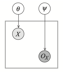
We have that \begin{align} &P(X=1)=\theta,&&\hspace{1cm}P(x=0)=1-\theta \\ &P(O_X=o^1)=\psi,&&\hspace{1cm}P(O_X=o^0)=1-\psi \end{align} and thus \begin{align} P(Y=1)&=\theta\psi \\ P(Y=0)&=(1-\theta)\psi \\ P(Y=?)&=1-\psi \end{align} Thus if we see a dataset $\mathcal{D}$ with $M[1],M[0]$ and $M[?]$ instances, then the likelihood is \begin{align} L(\theta,\psi:\mathcal{D})&=(\theta\psi)^{M[1]}\big((1-\theta)\psi\big)^{M[0]}(1-\psi)^{M[?]} \\ &=\theta^{M[1]}(1-\theta)^{M[0]}\psi^{M[1]+M[0]}(1-\psi)^{M[?]} \end{align} Differentiating the likelihood w.r.t $\theta$ and $\psi$ and setting the derivatives to zero we have that \begin{align} \hat{\theta}_\text{ML}&=\frac{M[1]}{M[1]+M[0]} \\ \hat{\psi}_\text{ML}&=\frac{M[1]+M[0]}{M[1]+M[0]+M[?]} \end{align}
Example 5: Consider the following observability model with $X\sim\text{Bern}(\theta)$, $(O_X\vert X=1)\sim\text{Bern}(\psi_{O_X\vert x^1})$ and $(O_X\vert X=0)\sim\text{Bern}(\psi_{O_X\vert x^0})$.
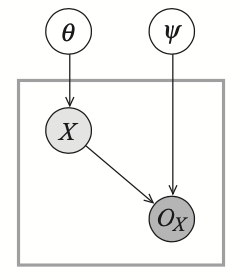
In this case, we have that \begin{align} &P(X=1)=\theta,&&\hspace{1cm}P(x=0)=1-\theta \\ &P(O_X=o^1\vert X=1)=\psi_{O_X\vert x^1},&&\hspace{1cm}P(O_X=o^0\vert X=1)=1-\psi_{O_X\vert x^1} \\ &P(O_X=o^1\vert X=0)=\psi_{O_X\vert x^0},&&\hspace{1cm}P(O_X=o^0\vert X=0)=1-\psi_{O_X\vert x^0} \end{align} and thus \begin{align} P(Y=1)&=\theta\psi_{O_X\vert x^1} \\ P(Y=0)&=(1-\theta)\psi_{O_X\vert x^0} \\ P(Y=?)&=\theta(1-\psi_{O_X\vert x^1})+(1-\theta)(1-\psi_{O_X\vert x^0}) \end{align} Then, given the dataset $\mathcal{D}$ with $M[1],M[0]$ and $M[?]$ examples, the likelihood function is given as \begin{align} &L(\theta,\psi_{O_X\vert x^1},\psi_{O_X\vert x^0}:\mathcal{D})\nonumber \\ &=(\theta\psi_{O_X\vert x^1})^{M[1]}\big[(1-\theta)\psi_{O_X\vert x^0}\big]^{M[0]}\big[\theta(1-\psi_{O_X\vert x^1})+(1-\theta)(1-\psi_{O_X\vert x^0})\big]^{M[?]} \end{align}
Decoupling of Observation Mechanism
Missing Completely At Random
A missing data model $P_\text{missing}$ is missing completely at random (MCAR) if $P_\text{missing}\models(\mathbf{X}\perp O_\mathbf{X})$.
In this case, the likelihood function of $X$ and $O_X$ decomposes as a product, and we can maximize each part separately. However, MCAR is sufficient but not necessary for the decomposition of the likelihood function.
Missing At Random
Let $\mathbf{y}$ be a tuple of observations. These observations partition the variables $\mathbf{X}$ into two sets
- the observed variables $\mathbf{X}_\text{obs}^\mathbf{y}=\{X_i:y_i\neq ?\}$;
- the hidden variables $\mathbf{X}_\text{hidden}^\mathbf{y}=\{X_i:y_i=?\}$.
The observations $\mathbf{y}$ determines the values of the observed variables, but not the hidden ones.
A missing data model $P_\text{missing}$ is missing at random (MAR) if for all observations $\mathbf{y}$ with $P_\text{missing}(\mathbf{y})>0$, and for all $\mathbf{x}_\text{hidden}^\mathbf{y}\in\text{Val}(\mathbf{X}_\text{hidden}^\mathbf{y})$, we have that \begin{equation} P_\text{missing}\models(o_\mathbf{X}\perp\mathbf{x}_\text{hidden}^\mathbf{y}\vert\mathbf{x}_\text{obs}^\mathbf{y}), \end{equation} where $o_\mathbf{X}$ are specific values of the observation variables given $\mathbf{Y}$.
This implies that given the observed variables, the observation pattern does not give any additional information about the hidden variables \begin{equation} P_\text{missing}(\mathbf{x}_\text{hidden}^\mathbf{y}\vert\mathbf{x}_\text{obs}^\mathbf{y},o_\mathbf{X})=P_\text{missing}(\mathbf{x}_\text{hidden}^\mathbf{y}\vert\mathbf{x}_\text{obs}^\mathbf{y}) \end{equation} Thus, with a missing model satisfying MAR, we have \begin{align} P_\text{missing}(\mathbf{y})&=P_\text{missing}(o_\mathbf{X},\mathbf{x}_\text{obs}^\mathbf{y}) \\ &=\sum_{\mathbf{x}_\text{hidden}^\mathbf{y}}\Big[P(\mathbf{x}_\text{obs}^\mathbf{y},\mathbf{x}_\text{hidden}^\mathbf{y})P_\text{missing}(o_\mathbf{X}\vert\mathbf{x}_\text{obs}^\mathbf{y},\mathbf{x}_\text{hidden}^\mathbf{y})\Big] \\ &=\sum_{\mathbf{x}_\text{hidden}^\mathbf{y}}\Big[P(\mathbf{x}_\text{obs}^\mathbf{y},\mathbf{x}_\text{hidden}^\mathbf{y})P_\text{missing}(o_\mathbf{X}\vert\mathbf{x}_\text{obs}^\mathbf{y})\Big] \\ &=P_\text{missing}(o_\mathbf{X}\vert\mathbf{x}_\text{obs}^\mathbf{y})\sum_{\mathbf{x}_\text{hidden}^\mathbf{y}}P(\mathbf{x}_\text{obs}^\mathbf{y},\mathbf{x}_\text{hidden}^\mathbf{y}) \\ &=P_\text{missing}(o_\mathbf{X}\vert\mathbf{x}_\text{obs}^\mathbf{y})P(\mathbf{x}_\text{obs}^\mathbf{y}),\label{eq:mar.1} \end{align} where the first equality is justified due to the fact that $\mathbf{y}$ are completely determined once we have the knowledge about $\mathbf{x}_\text{obs}^\mathbf{y}$ and $o_\mathbf{X}$.
Notice that the first term in \eqref{eq:mar.1}, $P_\text{missing}(o_\mathbf{X}\vert\mathbf{x}_\text{obs}^\mathbf{y})$, depends only on the parameters $\boldsymbol{\psi}$; while the second one, $P(\mathbf{x}_\text{obs}^\mathbf{y})$, depends only the parameters $\boldsymbol{\theta}$. And since we have this product for every observed instance, we then have the following result.
Theorem 3: If $P_\text{missing}$ satisfies MAR, then $L(\boldsymbol{\theta},\boldsymbol{\psi}:\mathcal{D})$ can be written as a product of two likelihood functions $L(\boldsymbol{\theta}:\mathcal{D})$ and $L(\boldsymbol{\psi}:\mathcal{D})$.
The Likelihood Function
Given a Bayesian network structure $\mathcal{G}$ over a set of variables $\mathbf{X}$, and dataset $\mathcal{D}$ of $M$ training instances, each of which has
- a different set of observed variables, denoted $\{\mathbf{O}[m]:m=1,\ldots,M\}$ and their corresponding values $\{\mathbf{o}[m]:m=1,\ldots,M\}$;
- a different set of hidden (or latent) variables, denoted $\{\mathbf{H}[m]:m=1,\ldots,M\}$
The likelihood function, $L(\boldsymbol{\theta}:\mathcal{D})$, is defined as the probability of the observed variables in the data, marginalizing the hidden variables, and ignoring the observability model: \begin{equation} L(\boldsymbol{\theta}:\mathcal{D})=\prod_{m=1}^{M}P(\mathbf{o}[m];\boldsymbol{\theta})\label{eq:tlf.1} \end{equation} And thus the log-likelihood is given as \begin{equation} \ell(\boldsymbol{\theta}:\mathcal{D})=\sum_{m=1}^{M}\log P(\mathbf{o}[m];\boldsymbol{\theta}) \end{equation} This definition of likelihood function suggests that the problem of learning with partially observed data basically does not differ from the problem of learning with fully observed data. However, the computational complexity is bigger in this case and it requires the use of missing data. \begin{equation} L(\boldsymbol{\theta}:\mathcal{D})=\prod_{m=1}^{M}P(\mathbf{o}[m];\boldsymbol{\theta})=\prod_{m=1}^{M}\sum_{\mathbf{h}[m]}P(\mathbf{o}[m],\mathbf{h}[m];\boldsymbol{\theta}) \end{equation} And thus the log-likelihood can be computed by \begin{equation} \ell(\boldsymbol{\theta}:\mathcal{D})=\sum_{m=1}^{M}\log\sum_{\mathbf{h}[m]}P(\mathbf{o}[m],\mathbf{h}[m];\boldsymbol{\theta})\label{eq:tlf.2} \end{equation}
MLE
Gradient Ascent
Lemma 4: Let $\mathcal{B}$ be a Bayesian network with graph $\mathcal{G}$ over $\mathcal{X}$ that induces a probability distribution $P$, let $\mathbf{o}$ be a tuple of observations for some variables, and let $X\in\mathcal{X}$ be some r.v. If $P(x\vert\mathbf{u})>0$, where $x\in\text{Val}(X)$, $\mathbf{u}\in\text{Val}(\text{Pa}_X)$, then we have \begin{equation} \frac{\partial P(\mathbf{o})}{\partial P(x\vert\mathbf{u})}=\frac{P(x,\mathbf{u},\mathbf{o})}{P(x\vert\mathbf{u})} \end{equation}
Proof
Consider the case of full assignment $\xi$. We have
\begin{equation}
P(\xi)=\prod_{X_i\in\mathcal{X}}P(\xi\langle X_i\rangle\vert\xi\langle\text{Pa}_{X_i}\rangle)
\end{equation}
Thus, we have that
\begin{equation}
\hspace{-1cm}\frac{\partial P(\xi)}{\partial P(x\vert\mathbf{u})}=\begin{cases}\displaystyle\prod_{X_i\in\mathcal{X},X_i\neq X}P\big(\xi\langle X_i\rangle\vert\xi\langle\text{Pa}_{X_i}\rangle\big)=\frac{P(\xi)}{P(x\vert\mathbf{u})}&\hspace{1cm}\text{if }\xi\langle X,\text{Pa}_X\rangle=\langle x,\mathbf{u}\rangle \\ 0&\hspace{1cm}\text{otherwise}\end{cases}\label{eq:ga.1}
\end{equation}
Now consider the case of partial assignment $\xi$. We have
\begin{equation}
P(\mathbf{o})=\sum_{\xi:\xi\langle\mathbf{O}\rangle=\mathbf{o}}P(\xi)
\end{equation}
Using the result \eqref{eq:ga.1}, we then have that
\begin{align}
\frac{\partial P(\mathbf{o})}{\partial P(x\vert\mathbf{u})}&=\sum_{\xi:\xi\langle\mathbf{O}\rangle=\mathbf{o}}\frac{\partial P(\xi)}{\partial P(x\vert\mathbf{u})} \\ &=\sum_{\xi:\xi\langle\mathbf{O}\rangle=\mathbf{o},\xi\langle X,\text{Pa}_X\rangle=\langle x,\mathbf{u}\rangle}\frac{P(\xi)}{P(x\vert\mathbf{u})} \\ &=\frac{P(x,\mathbf{u},\mathbf{o})}{P(x\vert\mathbf{u})}
\end{align}
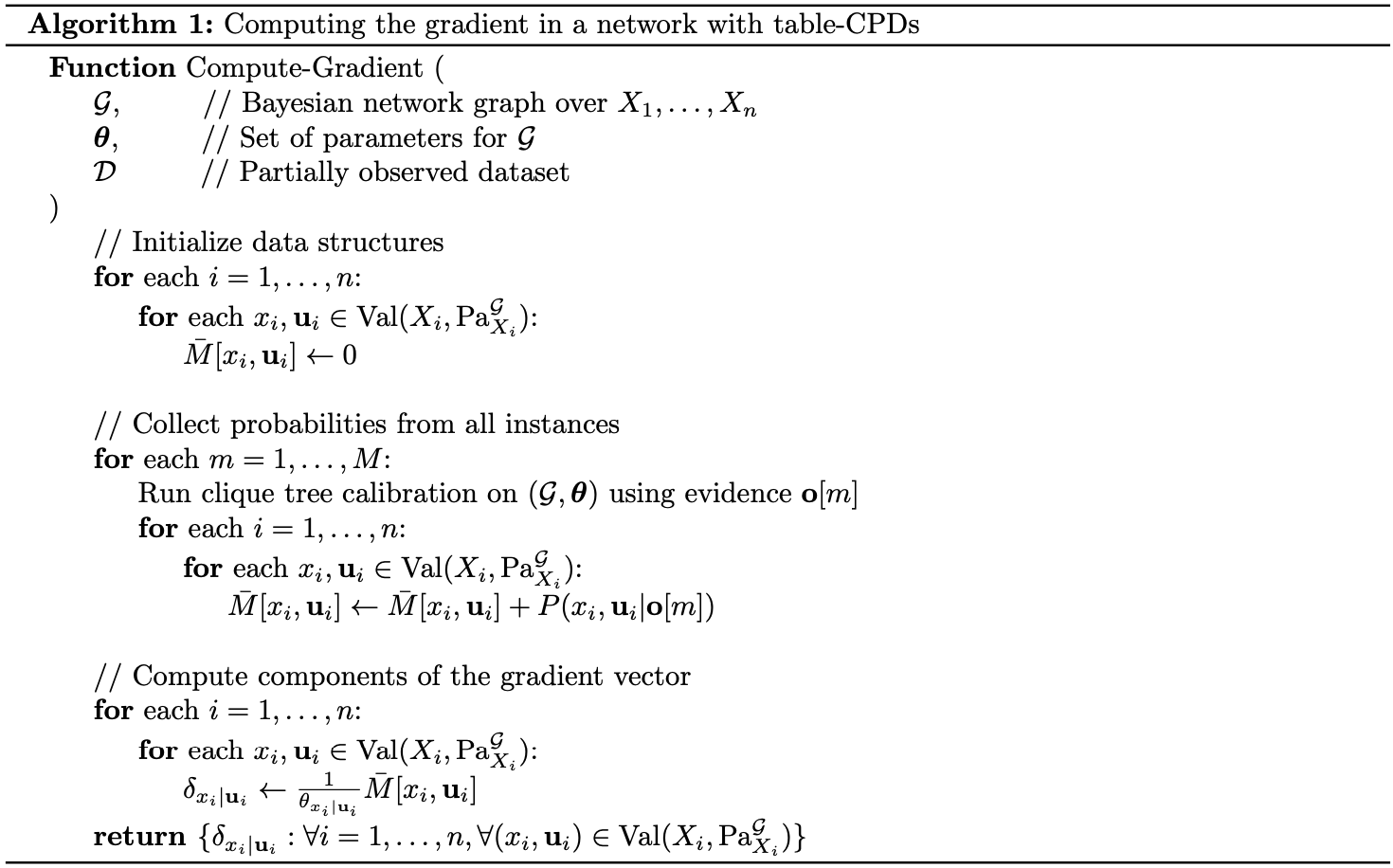
Given this result, we immediately obtain the form of the gradient of the likelihood function for table-CPDs.
Theorem 5: Let $\mathcal{G}$ be a Bayesian network graph over $\mathcal{X}$, and let $\mathcal{D}=\{\mathbf{o}[1],\ldots,\mathbf{o}[M]\}$ be a partially observable dataset. Let $X$ be a variable with parents $\mathbf{U}$ in $\mathcal{G}$. If $P(x\vert\mathbf{u})>0$, where $x\in\text{Val}(X)$, $\mathbf{u}\in\text{Val}(\mathbf{U})$, then we have \begin{equation} \frac{\partial\ell(\boldsymbol{\theta}:\mathcal{D})}{\partial P(x\vert\mathbf{u})}=\frac{1}{P(x\vert\mathbf{u})}\sum_{m=1}^{M}P(x,\mathbf{u}\vert\mathbf{o}[m];\boldsymbol{\theta}) \end{equation}
Proof
The gradient of the log-likelihood can be written as
\begin{align}
\frac{\partial\ell(\boldsymbol{\theta}:\mathcal{D})}{\partial P(x\vert\mathbf{u})}&=\sum_{m=1}^{M}\frac{\partial}{\partial P(x\vert\mathbf{u})}\log P(\mathbf{o}[m];\boldsymbol{\theta}) \\ &=\sum_{m=1}^{M}\frac{1}{P(\mathbf{o}[m];\boldsymbol{\theta})}\frac{\partial P(\mathbf{o}[m];\boldsymbol{\theta})}{\partial P(x\vert\mathbf{u})} \\ &=\sum_{m=1}^{M}\frac{1}{P(\mathbf{o}[m];\boldsymbol{\theta})}\frac{P(x,\mathbf{u},\mathbf{o}[m];\boldsymbol{\theta})}{P(x\vert\mathbf{u})} \\ &=\frac{1}{P(x\vert\mathbf{u})}\sum_{m=1}^{M}P(x,\mathbf{u}\vert\mathbf{o}[m];\boldsymbol{\theta})
\end{align}
where the third equality is obtained by applying Lemma 4.
Using this result, suppose that the CPDs entries of $P(X\vert\mathbf{U})$ are written as functions of some set of parameters $\boldsymbol{\theta}$. Then for a specific parameter $\theta\in\boldsymbol{\theta}$, we have \begin{equation} \frac{\partial\ell(\boldsymbol{\theta}:\mathcal{D})}{\partial\theta}=\sum_{x,\mathbf{u}}\frac{\partial\ell(\boldsymbol{\theta}:\mathcal{D})}{\partial P(x\vert\mathbf{u})}\frac{\partial P(x\vert\mathbf{u})}{\partial\theta} \end{equation}
Expectation Maximization
[TODO] Consider the following model, which is described by the following meta-network, where $X$ is fully observed, while $Z$ is partially observed.
The log-likelihood, as described in \eqref{eq:tlf.2}, is then given as \begin{align} \ell(\boldsymbol{\theta}:\mathcal{D})&=\sum_{m=1}^{M}\log P(x[m];\boldsymbol{\theta}) \\ &=\sum_{m=1}^{M}\log\sum_{z[m]}P(x[m],z[m];\boldsymbol{\theta}) \end{align} [TODO] For each $m=1,\ldots,M$, let $Q_m$ be some distribution over $Z$, i.e. $\sum_z Q_m(z)=1$ and $Q_m(z)\geq 0$1. We have \begin{align} \hspace{-0.5cm}\sum_{m=1}^{M}\log P(x[m];\boldsymbol{\theta})&=\sum_{m=1}^{M}\log\sum_{z[m]\in\text{Val}(Z)}P(x[m],z[m];\boldsymbol{\theta}) \\ &=\sum_{m=1}^{M}\log\sum_{z[m]\in\text{Val}(Z)}Q_m(z[m])\frac{P(x[m],z[m];\boldsymbol{\theta})}{Q_m(z[m])} \\ &\geq\sum_{m=1}^{M}\sum_{z[m]\in\text{Val}(Z)}Q_m(z[m])\log\left(\frac{P(x[m],z[m];\boldsymbol{\theta})}{Q_m(z[m])}\right),\label{eq:em.1} \end{align} where in the third step, we have used Jensen’s inequality. Specifically, since $\log(\cdot)$ is a strictly concave function, due to $(\log(x))’’=-1/x^2<0$, then by Jensen’s inequality, we have \begin{align} \log\left(\sum_{z[m]}Q_m(z[m])\frac{P(x[m],z[m];\boldsymbol{\theta})}{Q_m(z[m])}\right)&=\log\left(\mathbb{E}_{z[m]\sim Q_m}\left[\frac{P(x[m],z[m];\boldsymbol{\theta})}{Q_m(z[m])}\right]\right) \\ &\geq\mathbb{E}_{z[m]\sim Q_m}\left[\log\left(\frac{P(x[m],z[m];\boldsymbol{\theta})}{Q_m(z[m])}\right)\right] \\ &=\sum_{z[m]}Q_m(z[m])\log\left(\frac{P(x[m],z[m];\boldsymbol{\theta})}{Q_m(z[m])}\right), \end{align} where equality holds where \begin{equation} \frac{P(x[m],z[m];\boldsymbol{\theta})}{Q_m(z[m])}=\mathbb{E}_{z[m]\sim Q_m}\left[\frac{P(x[m],z[m];\boldsymbol{\theta})}{Q_m(z[m])}\right], \end{equation} with probability $1$. This implies that \begin{equation} \frac{P(x[m],z[m];\boldsymbol{\theta})}{Q_m(z[m])}=c, \end{equation} where $c$ is a constant w.r.t $z[m]$. Moreover, since $\sum_z Q_m(z)=1$, we then have \begin{equation} Q_m(z[m])\propto P(x[m],z[m];\boldsymbol{\theta}) \end{equation} And since $Q_m$ is a distribution, we further have that \begin{align} Q_m(z[m])&=\frac{P(x[m],z[m];\boldsymbol{\theta})}{\sum_z P(x[m],z;\boldsymbol{\theta})} \\ &=\frac{P(x[m],z[m];\boldsymbol{\theta})}{P(x[m];\boldsymbol{\theta})} \\ &=P(z[m]\vert x[m];\boldsymbol{\theta})\label{eq:em.3} \end{align}
Hence, the RHS of \eqref{eq:em.1} then gives us a lower bound of the log-likelihood function and that $\ell(\boldsymbol{\theta}:\mathcal{D})$ reaches this value if our selection of $Q_m$ satisfies the equation \eqref{eq:em.3}, i.e. $Q_m(Z)=P(Z\vert x[m];\boldsymbol{\theta})$.
Our goal is to find parameters $\boldsymbol{\theta}$ that maximizes the log-likelihood $\ell(\boldsymbol{\theta}:\mathcal{D})$
Repeat until convergence:
$\hspace{1cm}$(E-step) For each $m=1,\ldots,M$, set: \begin{equation*} Q_m(Z):=P(Z\vert x[m];\boldsymbol{\theta}) \end{equation*} $\hspace{1cm}$(M-step) Set: \begin{equation*} \boldsymbol{\theta}:=\underset{\boldsymbol{\theta}}{\text{argmax}}\sum_{m=1}^{M}\sum_{z[m]\in\text{Val}(Z)}Q_m(z[m])\log\frac{P(x[m],z[m];\boldsymbol{\theta})}{Q_m(z[m])} \end{equation*}
EM for Bayesian networks
Let us consider the EM algorithm for a general Bayesian network structure $\mathcal{G}$ with table-CPDs over random variables $X_1,\ldots,X_n$. Suppose that we are given a dataset $\mathcal{D}=\{\xi[1],\ldots,x[M]\}$, where for each instance $\xi[m]$, $\mathbf{O}[m]$ and $\mathbf{o}[m]$ denote the set of observed variables and their values, while $\mathbf{H}[m]$ represents the set of hidden variables. The log-likelihood function is given as \begin{align} \ell(\boldsymbol{\theta}:\mathcal{D})&=\sum_{m=1}^{M}\log P(\mathbf{o}[m];\boldsymbol{\theta}) \\ &=\sum_{m=1}^{M}\log\sum_{\mathbf{h}\in\text{Val}(\mathbf{H}[m])}P(\mathbf{o}[m],\mathbf{h};\boldsymbol{\theta}) \\ &\geq\sum_{m=1}^{M}\sum_{\mathbf{h}\in\text{Val}(\mathbf{H}[m])}Q_m(\mathbf{h})\log\frac{P(\mathbf{o}[m],\mathbf{h};\boldsymbol{\theta})}{Q_m(\mathbf{h})} \\ &=\left(\sum_{m=1}^{M}\sum_{\mathbf{h}\in\text{Val}(\mathbf{H}[m])}Q_m(\mathbf{h})\big[\log P(\mathbf{o}[m],\mathbf{h};\boldsymbol{\theta})-\log Q_m(\mathbf{h})\big]\right) \\ &=\sum_{m=1}^{M}\sum_{\mathbf{h}\in\text{Val}(\mathbf{H}[m])}Q_m(\mathbf{h})\log\prod_{i=1}^{n}P\Big(\xi[m]\langle X_i\rangle\Big\vert\xi[m]\langle\text{Pa}_{X_i}^\mathcal{G}\rangle;\boldsymbol{\theta}_{X_i\vert\text{Pa}_{X_i}^\mathcal{G}}\Big)\nonumber \\ &\hspace{1cm}+\sum_{m=1}^{M}H_{Q_m}(Q_m(\mathbf{H}[m])) \\ &=\sum_{m=1}^{M}\sum_{\mathbf{h}\in\text{Val}(\mathbf{H}[m])}Q_m(\mathbf{h})\sum_{i=1}^{n}\log P\Big(\xi[m]\langle X_i\rangle\Big\vert\xi[m]\langle\text{Pa}_{X_i}^\mathcal{G}\rangle;\boldsymbol{\theta}_{X_i\vert\text{Pa}_{X_i}^\mathcal{G}}\Big)\nonumber \\ &\hspace{1cm}+\sum_{m=1}^{M}H_{Q_m}(Q_m(\mathbf{H}[m])) \\ &=\sum_{i=1}^{n}\left(\sum_{m=1}^{M}\sum_{\mathbf{h}\in\mathbf{H}[m]}Q_m(\mathbf{h})\log P\Big(\xi[m]\langle X_i\rangle\Big\vert\xi[m]\langle\text{Pa}_{X_i}^\mathcal{G}\rangle;\boldsymbol{\theta}_{X_i\vert\text{Pa}_{X_i}^\mathcal{G}}\Big)\right)\nonumber \\ &\hspace{1cm}+\sum_{m=1}^{M}H_{Q_m}(Q_m(\mathbf{H}[m])) \\ &\triangleq\tilde{\ell}(\boldsymbol{\theta}) \end{align} This gives us a lower bound for the log-likelihood function $\ell(\boldsymbol{\theta}:\mathcal{D})$. And similarly, in the E-step of EM algorithm, for each $m=1,\ldots,M$, we set \begin{equation} Q_m(\mathbf{H})=P(\mathbf{H}\vert\mathbf{o}[m];\boldsymbol{\theta}) \end{equation} In the M-step of EM, we find a parameter $\boldsymbol{\theta}$ that maximizes $\tilde{\ell}(\boldsymbol{\theta})$. Before performing this step, we notice that the function $\tilde{\ell}(\boldsymbol{\theta})$ can be decomposed into sum of function of local CPDs $P(X_i\vert\text{Pa}_{X_i}^\mathcal{G};\boldsymbol{\theta}_{X_i\vert\text{Pa}_{X_i}^\mathcal{G}})$, which parameterized by $\boldsymbol{\theta}_{X_i\vert\text{Pa}_{X_i}^\mathcal{G}}$. Hence, as usual, we can independently solve for the local problems and then combine the solutions together.
In particular, during M-step, for each variable $X$, and for each $U\in\text{Pa}_X^\mathcal{G}$, we try to solve the optimization problem \begin{align} \underset{\boldsymbol{\theta}_{X\vert U}}{\text{maximize}}&\sum_{m=1}^{M}\sum_{\mathbf{h}\in\mathbf{H}[m]}Q_m(\mathbf{h})\log P\big(\xi[m]\langle X\rangle\big\vert\xi[m]\langle U\rangle;\boldsymbol{\theta}_{X\vert u}) \\ \text{s.t.}&\sum_{x\in\text{Val}(X)}\theta_{x\vert u}=1,\hspace{1cm}\forall u\in\text{Val}(U) \end{align} The Lagrangian of this problem is \begin{align} &\mathcal{L}(\boldsymbol{\theta}_{X\vert U},\lambda)\nonumber \\ &=-\sum_m\sum_\mathbf{h}Q_m(\mathbf{h})\log P\big(\xi[m]\langle X\rangle\big\vert\xi[m]\langle U\rangle;\boldsymbol{\theta}_{X\vert u})+\sum_{u\in\text{Val}(U)}\lambda_u\left(\sum_x\theta_{x\vert u}-1\right) \\ &=-\sum_m\sum_\mathbf{h}Q_m(\mathbf{h})\log\prod_{(x,u)\in\text{Val}(X,U)}\theta_{x\vert u}^{\mathbf{1}\{\xi[m]\langle X,U\rangle=\langle x,u\rangle\}}+\sum_u\lambda_u\left(\sum_x\theta_{x\vert u}-1\right) \\ &=-\sum_m\sum_\mathbf{h}Q_m(\mathbf{h})\sum_{x,u}\mathbf{1}\{\xi[m]\langle X,U\rangle=\langle x,u\rangle\}\log\theta_{x\vert u}+\sum_u\lambda_u\left(\sum_x\theta_{x\vert u}-1\right) \end{align} Differentiating w.r.t $\theta_{x\vert u}$ yields \begin{equation} \nabla_{\theta_{x\vert u}}\mathcal{L}(\boldsymbol{\theta}_{X\vert U},\lambda)=-\sum_m\sum_\mathbf{h}Q_m(\mathbf{h})\frac{\mathbf{1}\{\xi[m]\langle X,U\rangle=\langle x,u\rangle\}}{\theta_{x\vert u}}+\lambda_u \end{equation} Setting this derivative to zero, we obtain \begin{equation} \theta_{x\vert u}=\frac{1}{\lambda_u}\sum_m\sum_\mathbf{h}Q_m(\mathbf{h})\mathbf{1}\{\xi[m]\langle X,U\rangle=\langle x,u\rangle\}\triangleq\frac{f(x,u)}{\lambda_u} \end{equation} The dual function is then given as \begin{align} g(\lambda)&=\sup_{\boldsymbol{\theta}_{X\vert U}}\mathcal{L}(\boldsymbol{\theta}_{X\vert U},\lambda) \\ &=-\sum_{x,u}\log\left(\frac{f(x,u)}{\lambda_u}\right)f(x,u)+\sum_u\lambda_u\left(\sum_x\frac{f(x,u)}{\lambda_u}-1\right) \\ &=\sum_{x,u}\big(\log\lambda_u-\log f(x,u)\big)f(x,u)+\sum_{x,u}f(x,u)-\sum_u\lambda_u \end{align} Taking the derivative w.r.t $\lambda_u$ lets us obtain \begin{align} \frac{\partial g(\lambda)}{\partial\lambda_u}&=\sum_x\frac{f(x,u)}{\lambda_u}-1, \end{align} which gives us the value of $\lambda_u$ if being set to zero \begin{equation} \lambda_u=\sum_x f(x,u) \end{equation} Hence, we have the solution for $\theta_{x\vert u}$: \begin{align} \theta_{x\vert u}&=\frac{f(x,u)}{\sum_x f(x,u)} \\ &=\frac{\sum_m\sum_\mathbf{h}Q_m(\mathbf{h})\mathbf{1}\{\xi[m]\langle X,U\rangle=\langle x,u\rangle\}}{\sum_x\sum_m\sum_\mathbf{h}Q_m(\mathbf{h})\mathbf{1}\{\xi[m]\langle X,U\rangle=\langle x,u\rangle\}} \\ &=\frac{\sum_m\sum_\mathbf{h}P(\mathbf{h}\vert\mathbf{o}[m];\boldsymbol{\theta})\mathbf{1}\{\xi[m]\langle X,U\rangle=\langle x,u\rangle\}}{\sum_x\sum_m\sum_\mathbf{h}P(\mathbf{h}\vert\mathbf{o}[m];\boldsymbol{\theta})\mathbf{1}\{\xi[m]\langle X,U\rangle=\langle x,u\rangle\}} \\ &=\frac{\sum_m P(x,u\vert\mathbf{o}[m];\boldsymbol{\theta})}{\sum_x\sum_m P(x,u\vert\mathbf{o}[m];\boldsymbol{\theta})} \end{align} We end up with this pseudocode for EM in Bayesian network with table-CPDs.
Bayesian Learning
Structure Learning
References
[1] Daphne Koller, Nir Friedman. Probabilistic Graphical Models. The MIT Press, 2009.
[2] Christopher M. Bishop. Pattern Recognition and Machine Learning. Springer New York, NY, 2006.
[3] Stanford CS229. Machine Learning.
Footnotes
Without loss of generality, we have implicitly assumed that $Z$ is discrete. The same arguments can be extended to the continuous case by using integrations instead of summations. ↩︎