Read-through: Probabilistic Graphical Models - Inference

Notes on Inference in PGMs.

Exact Inference

Variable Elimination

Consider a simple chain $A\rightarrow B\rightarrow C\rightarrow D$ with our interest of computing $P(D)$, which can be computed by \begin{equation} P(D)=\sum_C\sum_B\sum_A P(A,B,C,D)\label{eq:int.1} \end{equation} This computation is ineffective, since it grows exponentially with the number of variables $n$. Specifically, if each of variables $A,B,C,D$ ($n=4$) takes $k$ possible values, the time complexity required is $\mathcal{O}(k^{n-1})$.

Using the chain rule of probability, we can instead calculate $P(D)$ as \begin{align} P(D)&=\sum_C\sum_B\sum_A P(A,B,C,D) \\ &=\sum_C P(D\vert C)\sum_B P(C\vert B)\color{red}{\sum_A P(A)P(B\vert A)} \\ &=\sum_C P(D\vert C)\color{red}{\sum_B P(C\vert B)P(B)} \\ &=\color{red}{\sum_C P(D\vert C)P(C)}, \end{align} which has computation cost of $\mathcal{O}((n-1)k(k-1))=\mathcal{O}(nk^2)$ only due to each $\color{red}{summation}$ takes $k(k-1)$ computations.

Remark: The later computation is more effective than the former one due to

• The local independencies in Bayesian networks allow us to compactly rewrite $P(X\vert\mathcal{X}\backslash X)=P(X\vert\text{Pa}_X)$.
• At each step, by computing the $\color{red}{summations}$ first, we cached their values to use in the outer summations.

Basic Elimination

As in Representation task, using the notion of factors, we then can formally define an algorithm that applies to both Bayesian networks and Markov networks.

Factor Marginalization

Let $\mathbf{X}$ be a set of variables, and $Y\notin\mathbf{X}$. Let $\phi(\mathbf{X},Y)$ be a factor. By marginalizing out $Y$, we obtain the factor marginalization of $Y$ in $\phi$, which is a factor $\psi$ over $\mathbf{X}$ that \begin{equation} \psi(\mathbf{X})=\sum_Y\phi(\mathbf{X},Y) \end{equation} In addition, let us recall some useful identities of factors:

• Commutative of products: $\phi_1\cdot\phi_2=\phi_2\cdot\phi_1$.
• Commutative of summations: $\sum_X\sum_Y\phi=\sum_Y\sum_X\phi$.
• Associative of products: $(\phi_1\cdot\phi_2)\cdot\phi_3=\phi_1\cdot(\phi_2\cdot\phi_3)$.
• If $X\notin\text{Scope}(\phi_1)$, then \begin{equation} \sum_X(\phi_1\cdot\phi_2)=\phi_1\cdot\sum_X\phi_2\label{eq:fm.1} \end{equation}

The Variable Elimination Algorithm

Using identity \eqref{eq:fm.1}, we can write \begin{equation} P(A,B,C,D)=\phi_A\cdot\phi_B\cdot\phi_C\cdot\phi_D, \end{equation} which allows us to continue deriving \eqref{eq:int.1} as \begin{align} P(D)&=\sum_C\sum_B\sum_A P(A,B,C,D) \\ &=\sum_C\sum_B\sum_A\phi_A\cdot\phi_B\cdot\phi_C\cdot\phi_D \\ &=\sum_C\sum_B\phi_C\cdot\phi_D\cdot\left(\sum_A\phi_A\cdot\phi_B\right) \\ &=\sum_C\phi_D\cdot\left(\sum_B\phi_C\cdot\left(\sum_A\phi_A\cdot\phi_B\right)\right), \end{align} which is justified by the limited scope of the CPD factors, e.g. the second step is due to the fact that $A\notin\text{Scope}(\phi_C)\cup\text{Scope}(\phi_D)$. This computation suggests that in general, our problem is to computing the value of an expression of the form \begin{equation} \sum_\mathbf{Z}\prod_{\phi\in\Phi}\phi, \end{equation} which is referred as the sum-product inference task. This gives rise to the algorithm called Sum-Product Variable Elimination, as given in the following pseudocode.

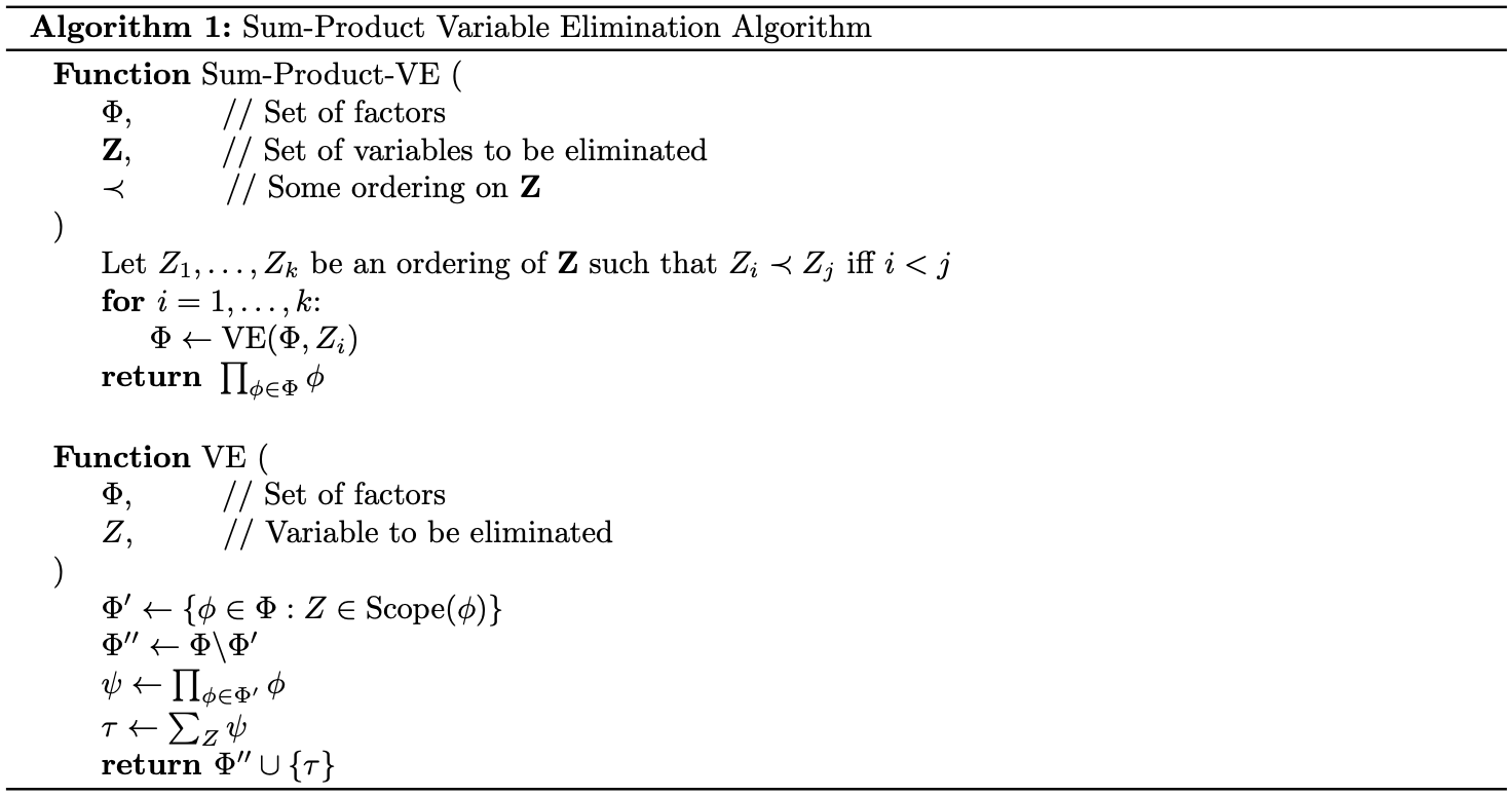
Theorem 1: Let $\mathbf{X}$ be some set of variables, and let $\Phi$ be a set of factors such that for each $\phi\in\Phi$, $\text{Scope}(\phi)\subset\mathbf{X}$. Let $\mathbf{Y}\subset\mathbf{X}$ be a set of query variables, and let $\mathbf{Z}=\mathbf{X}\backslash\mathbf{Y}$. Then for any ordering $\prec$ over $\mathbf{Z}$, $\text{Sum-Product-VE}(\Phi,\mathbf{Z},\prec)$ returns a factor $\phi^*(\mathbf{Y})$ such \begin{equation} \phi^*(\mathbf{Y})=\sum_\mathbf{Z}\prod_{\phi\in\Phi}\phi \end{equation} Remark:

• To apply the algorithm to a Bayesian network $\mathcal{B}$ for computing $P_\mathcal{B}(\mathbf{Y})$, we begin by instantiating $\Phi$ to comprise all of the CPDs \begin{equation} \Phi=\{\phi_{X_i}\}_{i=1,\ldots,n}, \end{equation} where $\phi_{X_i}=P(X_i\vert\text{Pa}_{X_i})$. Then, we apply the algorithm to the set $\mathbf{Z}=\mathcal{X}\backslash\mathbf{Y}$.
• Similarly, with a Markov network $\mathcal{H}$, we begin by instantiating $\Phi$ as the set of potential functions \begin{equation} \Phi=\{\phi_c\}_{c\in C}, \end{equation} where $C$ be a set of cliques of $\mathcal{H}$. Analogously, we then apply the algorithm to the set $\mathbf{Z}=\mathcal{X}\backslash\mathbf{Y}$, which now returns an unnormalized factor over $\mathbf{Y}$. By dividing the partition function, we obtain $P_\mathcal{H}(\mathbf{Y})$.

Example 1: Consider the following Bayesian network with the goal is to compute the probability that the student got the job.

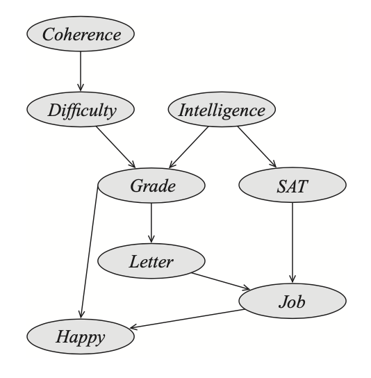
By chain rule of probability, we have that \begin{align} P(C,D,I,G,S,L,J,H)&=P(C)P(D\vert C)P(I)P(G\vert D,I)P(S\vert I)P(L\vert G)\nonumber \\ &\hspace{2cm}P(J\vert L,S)P(H\vert G,J) \\ &=\phi_C(C)\phi_D(D,C)\phi_I(I)\phi_G(G,D,I)\phi_S(S,I)\phi_L(L,G)\nonumber \\ &\hspace{2cm}\phi_J(J,L,S)\phi_H(H,G,J) \end{align} Consider the ordering: $C,D,I,H,G,S,L$. We step by step do the elimination procedure to each variable

• Eliminating $C$. We have \begin{align} \psi_1(D,C)&=\phi_C(C)\cdot\phi_D(D,C) \\ \tau_1(D)&=\sum_C\psi_1(D,C) \end{align}
• Eliminating $D$. We have \begin{align} \psi_2(G,D,I)&=\phi_G(G,D,I)\cdot\tau_1(D) \\ \tau_2(G,I)&=\sum_{D}\psi_2(G,D,I) \end{align}
• Eliminating $I$. We have \begin{align} \psi_3(G,I,S)&=\phi_I(I)\cdot\phi_S(S,I)\cdot\tau_2(G,I) \\ \tau_3(G,S)&=\sum_I\psi_3(G,I,S) \end{align}
• Eliminating $H$. We have \begin{align} \psi_4(H,G,J)&=\phi_H(H,G,J) \\ \tau_4(G,J)&=\sum_H\psi_4(H,G,J), \end{align} which is equal to $1$, since $\sum_H P(H\vert G,J)=1$
• Eliminating $G$. We have \begin{align} \psi_5(G,J,L,S)&=\phi_L(L,G)\cdot\tau_3(G,S)\cdot\tau_4(G,J) \\ \tau_5(L,S,J)&=\sum_G\psi_5(G,J,L,S) \end{align}
• Eliminating $S$. We have \begin{align} \psi_6(J,L,S)&=\phi_J(J,L,S)\cdot\tau_5(L,S,J) \\ \tau_6(J,L)&=\sum_S\psi_6(J,L,S) \end{align}
• Eliminating $L$. We have \begin{align} \psi_7(J,L)&=\tau_6(J,L) \\ \tau_7(J)&=\sum_L\psi_7(J,L) \end{align}

Semantics of Factors

Consider a factor produced as a product of some of the CPDs in a Bayesian network $\mathcal{B}$ \begin{equation} \tau(\mathbf{W})=\prod_{i=1}^{k}P(Y_i\vert\text{Pa}_{Y_i}), \end{equation} where \begin{equation} \mathbf{W}=\bigcup_{i=1}^{k}(\{Y_i\}\cup\text{Pa}_{Y_i}) \end{equation} Then, we can construct a Bayesian network $\mathcal{B}’$ and a disjoint partition $\mathbf{W}=\mathbf{Y}\cup\mathbf{Z}$ such that \begin{equation} \tau(\mathbf{W})=P_{\mathcal{B}’}(\mathbf{Y}\vert\mathbf{Z}) \end{equation}

Dealing with Evidence

Recall that by Proposition 17, we can view an unnormalized measure derived from introducing evidence into a Bayesian network as a Gibbs distribution.

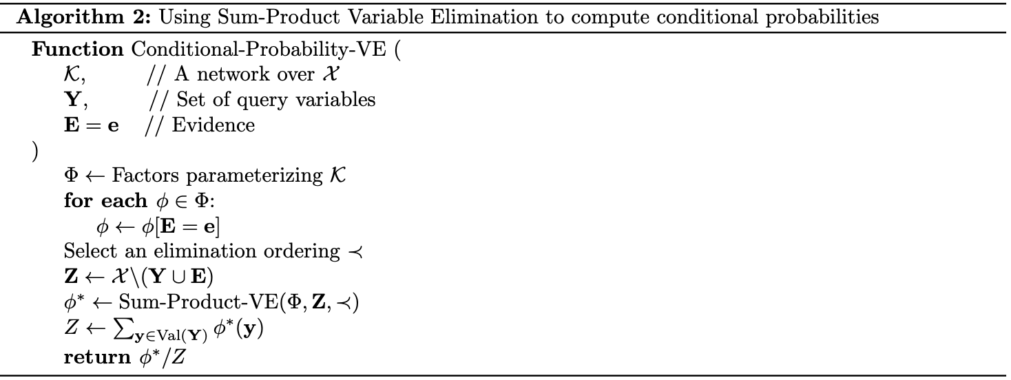
This suggests that in order to compute $P(\mathbf{Y}\vert\mathbf{e})$, we can apply the VE process to the set of factors in the network, reduced by $\mathbf{E}=\mathbf{e}$, and eliminate the variables in $\mathcal{X}\backslash(\mathbf{Y}\cup\mathbf{E})$.

The procedure outputs a factor $\phi^*(\mathbf{Y})$, which is exactly $P(\mathbf{Y},\mathbf{e})$. Normalizing this unnormalized distribution by dividing it with $\sum_\mathbf{Y}\phi^*(\mathbf{Y})$, which is precisely $P(\mathbf{e})$, we obtain $P(\mathbf{Y}\vert\mathbf{e})$.

Details for our overall procedure is given below, named as $\text{Conditional-Probability-VE}$.

Graph Structure of Variable Elimination

Graph Structure

Since the inputs to $\text{Sum-Product-VE}$ is a set of factors $\Phi$, set of variables to eliminated $\mathbf{Z}$ with some ordering $\prec$, the algorithm does take into account whether the graph generating factors is directed, undirected or partly directed. Hence, it is simplest to consider the algorithm as acting on an undirected graph $\mathcal{H}$.

Let $\Phi$ be a set of factors, we define \begin{equation} \text{Scope}(\Phi)\doteq\bigcup_{\phi\in\Phi}\text{Scope}(\phi) \end{equation} to be the set of all variables appearing in any of the factors in $\Phi$. We define $\mathcal{H}_\Phi$ to be the undirected graph whose nodes correspond to variables in $\text{Scope}(\Phi)$ and where we have an edge $X_i-X_j\in\mathcal{H}_\Phi$ iff there exists a factor $\phi\in\Phi$ such that $X_i,X_j\in\text{Scope}(\phi)$.

In other words, $\mathcal{H}_\Phi$ introduces a fully connected subgraph over the scope of each factor $\phi\in\Phi$. Hence, $\mathcal{H}_\Phi$ the minimal I-map for the distribution induced by $\Phi$.

Proposition 2: Let $P$ be a distribution defined by multiplying the factors in $\Phi$ then normalizing, i.e. let $\mathbf{X}=\text{Scope}(\Phi)$, \begin{equation} P(\mathbf{X})=\frac{1}{Z}\prod_{\phi\in\Phi}\phi, \end{equation} where \begin{equation} Z=\sum_\mathbf{X}\prod_{\phi\in\Phi}\phi \end{equation} Then $\mathcal{H}_\Phi$ is the minimal Markov network I-map for $P$, and $\Phi$ is a parameterization of this network that defines the distribution $P$.

Proof
This follows directly from Theorem 16.

Remark: Using the arguments specified when converting from Bayesian networks to Markov networks, it is worth remarking that

• For a set of factors $\Phi$ defined by a Bayesian network $\mathcal{G}$ (in this case, the partition function $Z=1$), $\mathcal{H}_\Phi$ is exactly the moralized graph of $\mathcal{G}$.
• In more specific, $\mathcal{H}_\Phi$ is the Markov network induced by a set of factors $\Phi[\mathbf{e}]$ defined by the reduction of the factors in a Bayesian network to some context $\mathbf{E}=\mathbf{e}$. In this case,
  • $\mathbf{X}=\text{Scope}(\Phi[\mathbf{e}])=\mathcal{X}\backslash\mathbf{E}$;
  • the unnormalized product of factors is $P(\mathbf{X},\mathbf{e})$;
  • the partition function is $P(\mathbf{e})$.

The Induced Graph

Let $\Phi$ be a set of factors over $\mathcal{X}=\{X_1,\ldots,X_n\}$ and let $\prec$ be an elimination ordering for some $\mathbf{X}\subset\mathcal{X}$. The induced graph $\mathcal{I}_{\Phi,\prec}$ is an undirected graph over $\mathcal{X}$, where $X_i$ and $X_j$ are connected via an edge if they both appear in some intermediate factor $\psi$ generated by VE using $\prec$ as an elimination ordering.

Theorem 3: Let $\mathcal{I}_{\Phi,\prec}$ be the induced graph for a set of factor $\Phi$ and some elimination ordering $\prec$. Then:

• The scope of every factor generated during the VE process is a clique in $\mathcal{I}_{\Phi,\prec}$.
• Every maximal clique in $\mathcal{I}_{\Phi,\prec}$ is the scope of some intermediate factor in the computation.

Proof

• Consider a factor $\psi(Y_1,\ldots,Y_k)$ generated during the VE procedure. By definition of the induced graph, there must be an edge between each pair $(Y_i,Y_j)$, which implies that $Y_1,\ldots,Y_k$ form a clique.

Induced Width, Tree-width

The width, denoted $w$, of an induced graph is the number of nodes in the largest clique in the graph minus $1$.

The induced width $w_{\mathcal{K},\prec}$ of an ordering $\prec$ relative to a graph $\mathcal{K}$ (directed or undirected) is defined to be the width of the graph $\mathcal{I}_{\mathcal{I},\prec}$ induced by applying VE to $\mathcal{K}$ using the ordering $\prec$.

The tree-width of a graph $\mathcal{K}$ is defined to be its minimal induced width \begin{equation} w_\mathcal{K}^*=\min_\prec w(\mathcal{I}_{\mathcal{K},\prec}) \end{equation}

Clique Trees

Variable Elimination and Clique Trees

Recall that in each elimination step of the VE process, a factor $\psi_i$ is introduced as the product of existing factors. Then, by marginalizing $\psi_i$, we eliminate a variable to create a new factor $\tau_i$, which is then used to introduce another factor $\psi_j$, and $\tau_j$ afterward and so on.

Let us consider $\psi_j$ be a computational data structure, which takes $\tau_i$, which we refer as a message, generated by other factor $\psi_i$, and generates a message $\tau_j$ that is used by another factor $\psi_l$.

Cluster Graphs

A cluster graph $\mathcal{U}$ for a set of factors $\Phi$ over $\mathcal{X}$ is an undirected graph, each of whose nodes $i$ is associated with a subset $\mathbf{C}_i\subset\mathcal{X}$.

A cluster graph must be family preserving, i.e. each factor $\phi\in\Phi$ must be associated with a cluster $\mathbf{C}_i$, denoted $\alpha(\phi)$, such that $\text{Scope}(\phi)\subset\mathbf{C}_i$.

Each edge between a pair of cluster $\mathbf{C}_i$ and $\mathbf{C}_j$ is associated with a sepset $\mathbf{S}_{i,j}\subset\mathbf{C}_i\cap\mathbf{C}_j$.

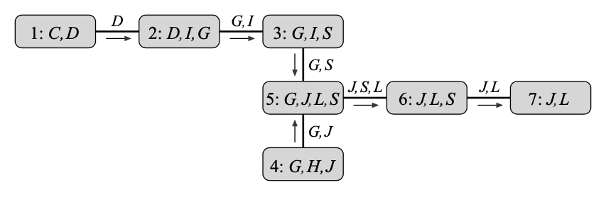
Example 2: Consider the execution of VE in Example 1, with its elimination ordering, we can define a cluster graph whose nodes and edges are given by:

• We have $\mathbf{C}_i=\text{Scope}(\psi_i)$. In particular, \begin{align} \mathbf{C}_1&=\text{Scope}(\psi_1)=\{C,D\} \\ \mathbf{C}_2&=\text{Scope}(\psi_2)=\{D,I,G\} \\ \mathbf{C}_3&=\text{Scope}(\psi_3)=\{G,I,S\} \\ \mathbf{C}_4&=\text{Scope}(\psi_4)=\{G,H,J\} \\ \mathbf{C}_5&=\text{Scope}(\psi_5)=\{G,J,L,S\} \\ \mathbf{C}_6&=\text{Scope}(\psi_6)=\{J,L,S\} \\ \mathbf{C}_7&=\text{Scope}(\psi_7)=\{J,L\} \end{align}
• We have an edge between two cluster $\mathbf{C}_i$ and $\mathbf{C}_j$ if the message $\tau_i$, produced by eliminating a variable in $\psi_i$, is used in the production of $\tau_j$.

We thus have the following cluster graph.

Remark: It is worth noticing that

• The VE algorithm uses each intermediate factor $\tau_i$ at most once. Specifically, when $\phi_i$ is used to produce $\psi_i$, it is removed from the set of factors $\Phi$, and thus cannot be used again. Therefore, the cluster graph induced by VE is a tree.
• Although a cluster graph is undirected, the execution of VE on it does define a directed graph induced by the flow of messages between the clusters. And thus, the induced directed graph is a directed tree with all the messages flowing toward a single cluster where the final result is computed. This cluster is known as the root of the tree.
• As a directed tree, we can define the notion of upstream and downstream in the sense that $\mathbf{C}_i$ is said to be upstream from $\mathbf{C}_j$, which is equivalent to saying that $\mathbf{C}_j$ is downstream from $\mathbf{C}_i$ if $\mathbf{C}_i$ is on the path from $\mathbf{C}_j$ to the root.

Clique Trees

Let $\mathcal{T}$ be a cluster tree over a set of factor $\Phi$, and let $\mathcal{V}_\mathcal{T}$ and $\mathcal{E}_\mathcal{T}$ denote its vertices and edges respectively. Then $\mathcal{T}$ is said to have the running intersection property if whenever there is a variable $X$ such that $X\in\mathbf{C}_i$ and $X\in\mathbf{C}_j$, then $X$ is also in every cluster in the (unique) path in $\mathcal{T}$ between $\mathbf{C}_i$ and $\mathbf{C}_j$.

Remark: This property implies that $\mathbf{S}_{i,j}=\mathbf{C}_i\cup\mathbf{C}_j$.

Theorem 4: Let $\mathcal{T}$ be a cluster tree induced by the VE algorithm over some set of factors $\Phi$. Then $\mathcal{T}$ satisfies the running intersection property.

Proof
Let $\mathbf{C}_X$ be the cluster where $X$ is eliminated. Our claim follows if we can show that for any cluster $\mathbf{C}\neq\mathbf{C}_X$, such that $X\in\mathbf{C}$, then $X$ appears in every clique on the path between $\mathbf{C}$ and $\mathbf{C}_X$.

By assumption, we first notice that $\mathbf{C}_X$ is upstream from $\mathbf{C}$ because if not, $X$ will not appear in the domain of the factor in $\mathbf{C}$ due after the elimination of $X$ in $\mathbf{C}_X$, $\Phi$ have no factor containing $X$.

Also, since $X\in\mathbf{C}$ and $X$ is not eliminated in $\mathbf{C}$, for each cluster upstream from $\mathbf{C}$ to $\mathbf{C}_X$, we have that $X$ must be in their scope, until it is eliminated in $\mathbf{C}_X$, which makes no upstream from $\mathbf{C}_X$ contains $X$. Therefore, $X$ appears in all clusters between $\mathbf{C}$ and $\mathbf{C}_X$.

Proposition 5: Let $\mathcal{T}$ be a cluster tree induced by the VE process over some set of factors $\Phi$. Let $\mathbf{C}_i$ and $\mathbf{C}_j$ be two neighboring clusters, such that $\mathbf{C}_i$ passes the message $\tau_i$ to $\mathbf{C}_j$. Then $\text{Scope}(\tau_i)=\mathbf{C}_i\cup\mathbf{C}_j$.

Proof

Let $\Phi$ be a set of factors over $\mathcal{X}$. A cluster tree over $\Phi$ that satisfies the running intersection property is called a clique tree (or junction tree, or join tree). Clusters are then called cliques.

Theorem 6: Let $\mathcal{T}$ be a cluster tree over $\Phi$, and let $\mathcal{H}_\Phi$ be an undirected graph parameterized by $\Phi$. Then $\mathcal{T}$ satisfies the running intersection property iff for every sepset $\mathbf{S}_{i,j}$, we have that \begin{equation} \text{sep}_{\mathcal{H}_\Phi}(\mathbf{W}_{<(i,j)};\mathbf{W}_{<(j,i)}\vert\mathbf{S}_{i,j}), \end{equation} where $\mathbf{W}_{<(i,j)}$ is the set of all variables in the scope of clusters in the $\mathbf{C}_i$ side of the tree, and where $\mathbf{W}_{<(j,i)}$ denotes the set of all variables in the scope of clusters in the $\mathbf{C}_j$ side of the tree.

Message Passing: Sum Product

Clique-Tree Message Passing

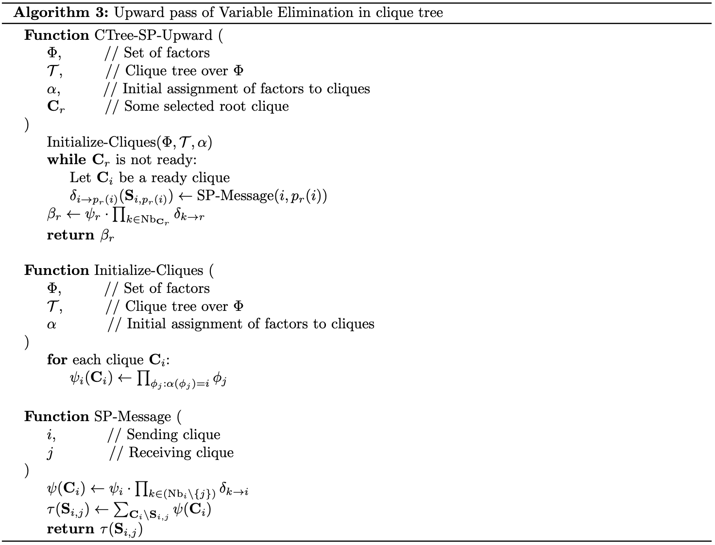
Let $\mathcal{T}$ be a clique tree with cliques $\mathbf{C}_1,\ldots,\mathbf{C}_k$. Since each factor $\phi\in\Phi$ is associated with some clique $\alpha(\phi)$, we then define the initial potential of $\mathbf{C}_i$ to be \begin{equation} \psi_i(\mathbf{C}_i)=\prod_{\phi:\alpha(\phi)=i}\phi \end{equation} Because each factor is assigned to exactly one clique, we are guaranteed that \begin{equation} \prod_\phi\phi=\prod_{i=1}^{k}\psi_i \end{equation} Let $\mathbf{C}_r$ be the selected root clique. For each clique $\mathbf{C}_i$, let $\text{Nb}_i$ denote the set of indices of cliques that are neighbors of $\mathbf{C}_i$, and let $p_r(i)$ be the upstream neighbor of $i$.

This means that each clique $\mathbf{C}_i$, except for the root, performs a message passing computation and sends a message to its upstream neighbor $\mathbf{C}_{p_r(i)}$.

The message from $\mathbf{C}_i$ to $\mathbf{C}_j$ is computed via the sum-product message passing computation, which multiplies all incoming messages from $\mathbf{C}_i$’s neighbors (other than $\mathbf{C}_j$) with its initial clique potential $\psi_i$, resulting in a factor $\psi$ whose scope is $\mathbf{C}_i$ itself. Then it sums out all variables except those in the sepset between $\mathbf{C}_i$ and $\mathbf{C}_j$ to produce a factor as a message to $\mathbf{C}_i$. In particular, \begin{align} \psi(\mathbf{C}_i)&=\psi_i\cdot\prod_{k\in(\text{Nb}_i\backslash\{j\})}\delta_{k\rightarrow i} \\ \delta_{i\rightarrow j}&=\sum_{\mathbf{C}_i\backslash\mathbf{S}_{i,j}}\psi=\sum_{\mathbf{C}_i\backslash\mathbf{S}_{i,j}}\left(\psi_i\cdot\prod_{k\in(\text{Nb}_i\backslash\{j\})}\delta_{k\rightarrow i}\right) \end{align} The process proceeds until reaching the root clique, which then multiplies all incoming messages with its initial clique potential, $\psi_r$, resulting in a factor referred as the beliefs, denoted $\beta_r(\mathbf{C}_r)$. \begin{equation} \beta_r(\mathbf{C}_r)=\psi_r\cdot\prod_{k\in\text{Nb}_{\mathbf{C}_r}}\delta_{k\rightarrow r}, \end{equation} The overall process is summarized into the pseudocode below.

Algorithm Correctness

In this section, we will be proving that for a clique satisfying the family preserving and running intersection property, the return of Algorithm 3 is precisely the exact inference result, i.e. \begin{equation} \beta_r(\mathbf{C}_r)=\sum_{\mathcal{X}\backslash\mathbf{C}_r}\tilde{P}_\Phi(\mathcal{X})$ \end{equation} We start by proving a result.

Proposition 7: Assume that $X$ is eliminated when a message is sent from $\mathbf{C}_i$ to $\mathbf{C}_j$. Then $X$ does not appear anywhere in the tree on the $\mathbf{C}_j$ side of the edge $(i-j)$.

Proof
Assume that $X$ appears in some clique $\mathbf{C}_k$ that is on the $\mathbf{C}_j$ side of the tree. This implies that $\mathbf{C}_j$ is on the path from $\mathbf{C}_i$ to $\mathbf{C}_k$.
Hence, by running intersection property, since $X$ appears in both $\mathbf{C}_i$ and $\mathbf{C}_k$, we then have that $X\in\mathbf{C}_j$, contradicts to the assumption that $X$ is eliminated before coming to $\mathbf{C}_j$.

We continue by letting $\mathcal{F}_{\prec(i\rightarrow j)}$ denote the set of factors in the cliques on the $\mathbf{C}_i$-side of the edge and letting $\mathcal{V}_{\prec(i\rightarrow j)}$ present the set of variables appear on the $\mathbf{C}_i$-side but not in the sepset $\mathbf{S}_{i,j}$.

Theorem 8: Let $\delta_{i\rightarrow j}$ be a message from $\mathbf{C}_i$ to $\mathbf{C}_j$. Then \begin{equation} \delta_{i\rightarrow j}(\mathbf{S}_{i,j})=\sum_{\mathcal{V}_{\prec(i\rightarrow j)}}\prod_{\phi\in\mathcal{F}_{\prec(i\rightarrow j)}}\phi\label{eq:ac.1} \end{equation}

Proof
We consider two cases:

• If the clique $\mathbf{C}_i$ is a leaf node of the clique tree, then $\mathbf{C}_j$ is the only clique connected to $\mathbf{C}_i$. Thus, \eqref{eq:ac.1} is simply the marginalization over $\mathbf{C}_i\backslash\mathbf{S}_{i,j}$ of the product of the factors whose scope is $\mathbf{C}_i$, which we have known that is precisely the message to send to $\mathbf{C}_j$.
• If $\mathbf{C}_i$ is not a leaf of the clique tree, let $i_1,\ldots,i_m$ denote the indices of the neighboring cliques of $\mathbf{C}_i$ other than $\mathbf{C}_j$. Then by Proposition 7, for $k=1,\ldots,m$, we have that $\mathcal{V}_{\prec(i_k\rightarrow i)}$ are disjoint sets and that \begin{equation} \mathcal{V}_{\prec(i\rightarrow j)}=\mathbf{Y}_i\cup\left(\bigcup_{k=1}^{m}\mathcal{V}_{\prec(i_k\rightarrow i)}\right), \end{equation} where $\mathbf{Y}_i$ are variables that are eliminated at $\mathbf{C}_i$, which implies that $\mathbf{Y}_i=\mathbf{C}_i\backslash\mathbf{S}_{i,j}$. And analogously, for $k=1,\ldots,m$, we also have that $\mathcal{F}_{\prec(i_k\rightarrow i)}$ are disjoint and \begin{equation} \mathcal{F}_{\prec(i\rightarrow j)}=\mathcal{F}_i\cup\left(\bigcup_{k=1}^{m}\mathcal{F}_{\prec(i_k\rightarrow i)}\right), \end{equation} where $\mathcal{F}_i$ denotes the set of factors from which the initial potential of $\mathbf{C}_i$, $\psi_i$, is computed. Hence, we have that \begin{align} \hspace{-1.5cm}\sum_{\mathcal{V}_{\prec(i\rightarrow j)}}\prod_{\phi\in\mathcal{F}_{\prec(i\rightarrow j)}}\phi&=\sum_{\mathbf{Y}_i\cup\left(\bigcup_{k=1}^{m}\mathcal{V}_{\prec(i_k\rightarrow i)}\right)}\left[\prod_{\mathcal{F}_i\cup\left(\bigcup_{k=1}^{m}\mathcal{F}_{\prec(i_k\rightarrow i)}\right)}\phi\right] \\ &=\sum_{\mathbf{Y}_i}\sum_{\mathcal{V}_{\prec(i_1\rightarrow i)}}\ldots\sum_{\mathcal{V}_{\prec(i_m\rightarrow i)}}\left[\left(\prod_{\phi\in\mathcal{F}_i}\phi\right)\left(\prod_{\phi\in\mathcal{F}_{\prec(i_1\rightarrow i)}}\phi\right)\ldots\left(\prod_{\phi\in\mathcal{F}_{\prec(i_m\rightarrow i)}}\phi\right)\right] \\ &=\sum_{\mathbf{Y}_i}\left[\left(\prod_{\phi\in\mathcal{F}_i}\phi\right)\left(\sum_{\mathcal{V}_{\prec(i_1\rightarrow i)}}\prod_{\phi\in\mathcal{F}_{\prec(i_1\rightarrow i)}}\phi\right)\ldots\left(\sum_{\mathcal{V}_{\prec(i_m\rightarrow i)}}\prod_{\phi\in\mathcal{F}_{\prec(i_m\rightarrow i)}}\phi\right)\right] \\ &=\sum_{\mathbf{Y}_i}\left[\left(\prod_{\phi\in\mathcal{F}_i}\phi\right)\cdot\prod_{k=1}^{m}\left(\sum_{\mathcal{V}_{\prec(i_k\rightarrow i)}}\prod_{\phi\in\mathcal{F}_{\prec(i_k\rightarrow i)}}\phi\right)\right] \\ &=\sum_{\mathbf{Y}_i}\left[\psi_i\cdot\prod_{k=1}^{m}\delta_{i_k\rightarrow i}\right] \\ &=\delta_{i\rightarrow j} \end{align}

Given these results, we then can state that:
Corollary 9: Let $\mathbf{C}_r$ be the root in a clique tree, and assume that $\beta_r$ is computed as in Algorithm 3. Then \begin{equation} \beta_r(\mathbf{C}_r)=\sum_{\mathcal{X}\backslash\mathbf{C}_r}\tilde{P}_\Phi(\mathcal{X}) \end{equation}

Example 3: Consider the simplified clique tree $\mathcal{T}$ for the Student network given in Example 1

With the goal of computing $P(J)$, we need to execute the VE procedure so that $J$ is not eliminated. Hence, the root clique must contain $J$. Selecting $\mathbf{C}_5$ as our root clique, we apply Variable Elimination in $\mathcal{T}$ as following

• We begin by defining the initial potentials \begin{align} \psi_1(\mathbf{C}_1)&=\psi_1(C,D)=\phi_C(C)\cdot\phi_C(D,C) \\ \psi_2(\mathbf{C}_2)&=\psi_2(D,I,G)=\phi_G(D,I,G) \\ \psi_3(\mathbf{C}_3)&=\psi_3(G,I,S)=\phi_I(I)\cdot\phi_S(I,S) \\ \psi_4(\mathbf{C}_4)&=\psi_4(G,H,J)=\phi_H(G,H,J) \\ \psi_5(\mathbf{C}_5)&=\psi_5(G,J,L,S)=\phi_L(L,G)\cdot\phi_J(J,L,S) \end{align}
• Given the initial potentials for each clique $\mathbf{C}_i$, we can proceed as
  • In $\mathbf{C}_1$, we have \begin{equation} \delta_{1\rightarrow 2}=\sum_C\psi_1(C,D) \end{equation}
  • In $\mathbf{C}_2$, we have \begin{equation} \delta_{2\rightarrow 3}=\sum_D\psi_2(D,I,G)\cdot\delta_{1\rightarrow 2} \end{equation}
  • In $\mathbf{C}_3$, we have \begin{equation} \delta_{3\rightarrow 5}=\sum_I\psi_3(G,I,S)\cdot\delta_{2\rightarrow 3} \end{equation}
  • In $\mathbf{C}_4$, we have \begin{equation} \delta_{4\rightarrow 5}=\sum_H\psi_4(G,H,J) \end{equation}
  • In $\mathbf{C}_5$, we have \begin{equation} \beta_5(G,J,L,S)=\psi_5(G,J,L,S)\cdot\delta_{3\rightarrow 5}\cdot\delta_{4\rightarrow 5} \end{equation}
• The resulting factor $\beta_5(G,J,L,S)$ is precisely the distribution $P(G,J,L,S)$. Thus, by summing out $G,L,S$, we have \begin{equation} P(J)=\sum_{G,L,S}P(G,J,L,S)=\sum_{G,L,S}\beta_5(G,J,L,S) \end{equation}

Remark: The algorithm can applied both to inference in Bayesian and Markov networks. Specifically,

• For a Bayesian network $\mathcal{B}$ such that $\Phi$ are the CPDs in $\mathcal{B}$, reduced with some evidence $\mathbf{e}$, then we have \begin{equation} \beta_r(\mathbf{C}_r)=P_\mathcal{B}(\mathbf{C}_r,\mathbf{e}) \end{equation} As usual, normalizing this with partition function $P_\mathcal{B}(\mathbf{e})$ gives us $P_\mathcal{B}(\mathbf{C}_r)$.
• For a Markov network $\mathcal{H}$ having $\Phi$ as its potential cliques, then we have \begin{equation} \beta_r(\mathbf{C}_r)=\tilde{P}_\Phi(\mathbf{C}_r) \end{equation} Similarly, normalizing this with partition function, which is given by $\sum_{\mathbf{C}_r}\beta_r(\mathbf{C}_r)$, gives us $P_\Phi(\mathbf{C}_r)$.

Clique Tree Calibration

Consider the task of computing distribution over every r.v.s in the network, i.e. $P(X)$ for all $X\in\mathcal{X}$.

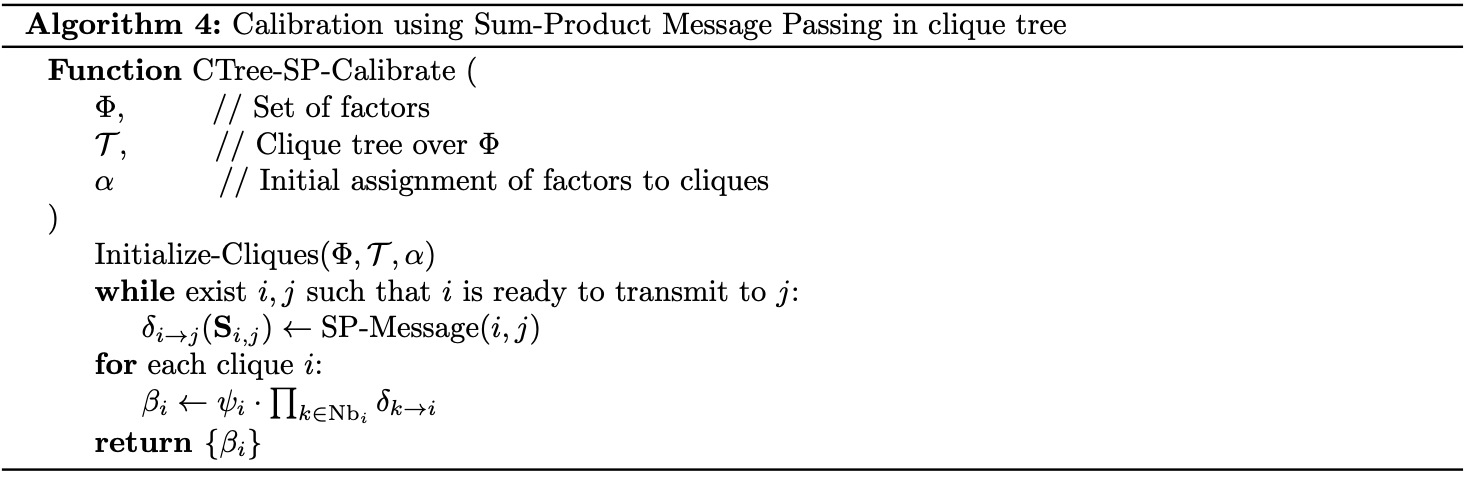
It follows from Theorem 8 that the message being sent from $\mathbf{C}_i$ to $\mathbf{C}_j$, $\delta_{i\rightarrow} j$, does not depend on the choice of root clique. Thus, each edge $(i-j)$ that connects $\mathbf{C}_i$ and $\mathbf{C}_j$ is associated with two messages $\delta_{i\rightarrow} j$ and $\delta_{j\rightarrow i}$.

Using this observation and based on Algorithm 3, we can develop an algorithm that effectively computes the beliefs for all cliques. It is then called Sum-Product Belief Propagation.

And thus, we have a result that directly follows from Corollary 9.

Corollary 10: Assume that, for each clique $i$, $\beta_i$ is computed via Algorithm 4. Then \begin{equation} \beta_i(\mathbf{C}_i)=\sum_{\mathcal{X}\backslash\mathbf{C}_i}\tilde{P}_\Phi(\mathcal{X}) \end{equation}

Calibrated

Recall that we can compute the marginal probability over a particular variable $X$ by selecting a clique containing $X$ in its scope, and summing out the other variables in the clique. Hence, each marginal probability over $X$ can be computed via multiples cliques, as long as their scope contains $X$. Or in other words, if $X$ appears in two cliques, they must agree on its marginal.

Two adjacent cliques $\mathbf{C}_i$ and $\mathbf{C}_j$ are calibrated if \begin{equation} \sum_{\mathbf{C}_i\backslash\mathbf{S}_{i,j}}\beta_i(\mathbf{C}_i)=\sum_{\mathbf{C}_j\backslash\mathbf{S}_{i,j}}\beta_j(\mathbf{C}_j) \end{equation} A clique tree $\mathcal{T}$ is said to be calibrated if all pairs of adjacent cliques are calibrated. \begin{equation} \sum_{\mathbf{C}_i\backslash\mathbf{S}_{i,j}}\beta_i(\mathbf{C}_i)=\sum_{\mathbf{C}_j\backslash\mathbf{S}_{i,j}}\beta_j(\mathbf{C}_j)\hspace{1cm}\forall(i-j)\in\mathcal{E}_\mathcal{T} \end{equation} In a calibrated clique tree, $\beta_i(\mathbf{C}_i)$ are referred as clique beliefs and the term sepset beliefs are known for \begin{equation} \mu_{i,j}(\mathbf{S}_{i,j})=\sum_{\mathbf{C}_i\backslash\mathbf{S}_{i,j}}\beta_i(\mathbf{C}_i)=\sum_{\mathbf{C}_j\backslash\mathbf{S}_{i,j}}\beta_j(\mathbf{C}_j) \end{equation} In words, after all the beliefs $\beta_i(\mathbf{C}_i)$ of the clique tree $\mathcal{T}$ is computed, then $\mathcal{T}$ is calibrated.

Calibrated Clique Trees as Distributions

Proposition 11: At convergence of the clique tree calibration algorithm, we have that \begin{equation} \tilde{P}_\Phi(\mathcal{X})=\frac{\prod_{i\in\mathcal{V}_\mathcal{T}}\beta_i(\mathbf{C}_i)}{\prod_{(i-j)\in\mathcal{E}_\mathcal{T}}\mu_{i,j}(\mathbf{S}_{i,j})}\label{eq:cctd.1} \end{equation}

Proof
By clique tree calibration algorithm, we have \begin{align} \frac{\prod_{i\in\mathcal{V}_\mathcal{T}}\beta_i(\mathbf{C}_i)}{\prod_{(i-j)\in\mathcal{E}_\mathcal{T}}\mu_{i,j}(\mathbf{S}_{i,j})}&=\frac{\prod_{i\in\mathcal{V}_\mathcal{T}}\left[\psi_i(\mathbf{C}_i)\prod_{k\in\text{Nb}_i}\delta_{k\rightarrow i}\right]}{\prod_{(i-j)\in\mathcal{E}_\mathcal{T}}\Big[\sum_{\mathbf{C}_i\backslash\mathbf{S}_{i,j}}\beta_i(\mathbf{C}_i)\Big]} \\ &=\frac{\left(\prod_{i\in\mathcal{V}_\mathcal{T}}\psi_i(\mathbf{C}_i)\right)\left(\prod_{(i-j)\in\mathcal{E}_\mathcal{T}}\delta_{i\to j}\delta_{j\to i}\right)}{\prod_{(i-j)\in\mathcal{E}_\mathcal{T}}\left[\sum_{\mathbf{C}_i\backslash\mathbf{S}_{i,j}}\left(\psi_i\delta_{j\to i}\prod_{k\in(\text{Nb}_i\backslash\{j\})}\delta_{k\to i}\right)\right]} \\ &=\frac{\left(\prod_{i\in\mathcal{V}_\mathcal{T}}\psi_i(\mathbf{C}_i)\right)\left(\prod_{(i-j)\in\mathcal{E}_\mathcal{T}}\delta_{i\to j}\delta_{j\to i}\right)}{\prod_{(i-j)\in\mathcal{E}_\mathcal{T}}\left[\delta_{j\to i}\sum_{\mathbf{C}_i\backslash\mathbf{S}_{i,j}}\left(\psi_i\prod_{k\in(\text{Nb}_i\backslash\{j\})}\delta_{k\to i}\right)\right]} \\ &=\frac{\left(\prod_{i\in\mathcal{V}_\mathcal{T}}\psi_i(\mathbf{C}_i)\right)\left(\prod_{(i-j)\in\mathcal{E}_\mathcal{T}}\delta_{i\to j}\delta_{j\to i}\right)}{\prod_{(i-j)\in\mathcal{E}_\mathcal{T}}\delta_{j\to i}\delta_{i\to j}} \\ &=\prod_{i\in\mathcal{V}_\mathcal{T}}\psi_i(\mathbf{C}_i)=\tilde{P}_\Phi(\mathcal{X}) \end{align} In other words, the clique beliefs $\{\beta_i(\mathbf{C}_i)\}_{i\in\mathcal{V}_\mathcal{T}}$ and sepset beliefs $\{\mu_{i,j}(\mathbf{S}_{i,j})\}_{(i-j)\in\mathcal{E}_\mathcal{T}}$ give us a reparameterization of the unnormalized measure $\tilde{P}_\Phi$. This property is known as the clique tree invariant.

Clique Tree Measure

Using the previous result, we can define the measure induced by a calibrated tree $\mathcal{T}$ to be \begin{equation} Q_\mathcal{T}=\frac{\prod_{i\in\mathcal{V}_\mathcal{T}}\beta_i(\mathbf{C}_i)}{\prod_{(i-j)\in\mathcal{E}_\mathcal{T}}\mu_{i,j}(\mathbf{S}_{i,j})}, \end{equation} where \begin{equation} \mu_{i,j}=\sum_{\mathbf{C}_i\backslash{S}_{i,j}}\beta_i(\mathbf{C}_i)=\sum_{\mathbf{C}_j\backslash{S}_{i,j}}\beta_j(\mathbf{C}_j) \end{equation}

Theorem 12: Let $\mathcal{T}$ be a clique tree over $\Phi$, and let $\beta_i(\mathbf{C}_i)$ be set of calibrated potentials for $\mathcal{T}$. Then $\tilde{P}_\Phi(\mathcal{X})\propto Q_\mathcal{T}$ iff for each $i\in\mathcal{V}_\mathcal{T}$, we have that \begin{equation} \beta_i(\mathbf{C}_i)\propto\tilde{P}_\Phi(\mathbf{C}_i) \end{equation}

Proof

• '$\Rightarrow$'
• '$\Leftarrow$'

Message Passing: Belief Update

Message Passing with Division

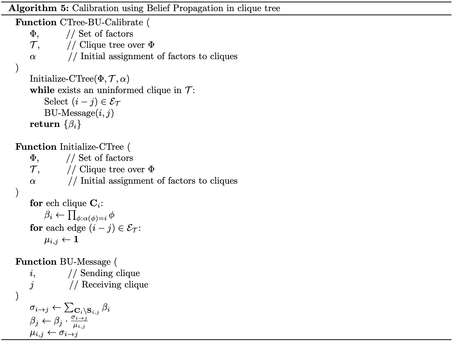
We first let $\mathbf{X}$ and $\mathbf{Y}$ be disjoint sets of variables, and let $\phi_1(\mathbf{X},\mathbf{Y})$ and $\phi_2(\mathbf{Y})$ be factors. The division $\frac{\phi_1}{\phi_2}$ is called a factor division which is a factor $\psi$ with scope $\mathbf{X},\mathbf{Y}$ given by \begin{equation} \psi(\mathbf{X},\mathbf{Y})=\frac{\phi_1(\mathbf{X},\mathbf{Y})}{\phi_2(\mathbf{Y})}, \end{equation} where we implicitly define $0/0=0$.

Recall that via calibration, the final potential (i.e. clique belief) at clique $i$ is computed by multiplying its initial potential, $\psi_i$ with the messages incoming from all of its neighbor, $\{\delta_{k\to i}\}_{k\in\text{Nb}_i}$: \begin{equation} \beta_i(\mathbf{C}_i)=\psi_i(\mathbf{C}_i)\prod_{k\in\text{Nb}_i}\delta_{k\to i} \end{equation} On the other hand, each message to send from $i$ to another clique $j$ computed by multiplying $\psi_i$ with the messages received from all of its neighbor except for $j$, $\{\delta_{k\to i}\}_{k\in(\text{Nb}_i\backslash\{j\})}$, and then marginalizing the clique $\mathbf{C}_i$ over the sepset $\mathbf{S}_{i,j}$ by summing out the variables on the non-sepset $\mathbf{C}_i\backslash\mathbf{S}_{i,j}$: \begin{align} \delta_{i\to j}(\mathbf{S}_{i,j})&=\sum_{\mathbf{C}_i\backslash\mathbf{S}_{i,j}}\psi_i(\mathbf{C}_i)\prod_{k\in(\text{Nb}_i\backslash\{j\})}\delta_{k\to i}(\mathbf{S}_{i,k}) \\ &=\sum_{\mathbf{C}_i\backslash\mathbf{S}_{i,j}}\frac{\beta_i(\mathbf{C}_i)}{\delta_{j\to i}(\mathbf{S}_{i,j})} \\ &=\frac{\sum_{\mathbf{C}_i\backslash\mathbf{S}_{i,j}}\beta_i(\mathbf{C}_i)}{\delta_{j\to i}(\mathbf{S}_{i,j})} \\ &=\frac{\mu_{i,j}(\mathbf{S}_{i,j})}{\delta_{j\to i}(\mathbf{S}_{i,j})} \end{align} This derivation gives rise to the sum-product-divide message passing scheme, where each clique $\mathbf{C}_i$ maintains its fully updated current beliefs $\beta_i=\psi_i\prod_{k\in\text{Nb}_i}\delta_{k\to i}$; while each sepset $\mathbf{S}_{i,j}$ also maintains its beliefs $\mu_{i,j}=\delta_{i\to j}\delta_{j\to i}$.

Equivalence of Sum-Product and Belief Update Messages

Theorem 13: In an execution of belief-update message passing, the clique tree invariant equation \eqref{eq:cctd.1} holds initially and after every message passing step.

Proof
At initialization, we have \begin{equation} \frac{\prod_{i\in\mathcal{V}_\mathcal{T}}\beta_i}{\prod_{(i-j)\in\mathcal{E}_\mathcal{T}}\mu_{i,j}}=\frac{\prod_{i\in\mathcal{V}_\mathcal{T}}\left[\prod_{\phi:\alpha(\phi)=i}\phi\right]}{\prod_{(i-j)\in\mathcal{E}_\mathcal{T}}1}=\frac{\prod_\phi\phi}{1}=\tilde{P}_\Phi\label{eq:espbu.1} \end{equation} For each $(i-j)\in\mathcal{E}_\mathcal{T}$, let $\beta_j’,\mu_{i,j}’$ be the beliefs returned after the message passing step, and let $\beta_j,\mu_{i,j}$ denote their previous values. The update rules in $\text{BU-Message}$ give us \begin{equation} \frac{\beta_j’}{\beta_j}=\frac{\mu_{i,j}’}{\mu_{i,j}}, \end{equation} which follows directly that the LHS of \eqref{eq:espbu.1} is unchanged after every step, and thus stays at $\tilde{P}_\Phi$.

Answering Queries

Constructing Clique Tree

Approximate Inference

Inference as Optimization

Exact Inference as Optimization

Assume we have a factorized distribution parameterized by set of factors $\Phi$: \begin{equation} P_\Phi(\mathcal{X})=\frac{1}{Z}\prod_{\phi\in\Phi}\phi(\mathbf{U}_\phi)\label{eq:eio.1} \end{equation} Recall that in exact inference, we find a set of calibrated beliefs that represent $P_\Phi(\mathcal{X})$, i.e. we find beliefs that match the distribution represented by given set of initial potentials.

Hence, we can view exact inference as searching over the set of distributions $\mathcal{Q}$ which are representable by the cluster tree to find a distribution $Q^*$ that matches $P_\Phi$. Or in other words, we are trying to search for a calibrated distribution that is as close as possible to $P_\Phi$. Thus, taking into account the KL divergence, or the relative entropy, between $Q$ and $P_\Phi$: \begin{equation} D_\text{KL}(Q\Vert P_\Phi)=\mathbb{E}_Q\left[\log\left(\frac{Q(\mathcal{X})}{P_\Phi(\mathcal{X})}\right)\right], \end{equation} our work is then to search for a distribution $Q$ that minimizes $D_\text{KL}(Q\Vert P_\Phi)$.

Specifically, let us assume that we are given a clique tree structure $\mathcal{T}$ for $P_\Phi$, i.e. $\mathcal{T}$ satisfies the family preserving and running intersection properties, and also assume that we are given a set of beliefs \begin{equation} \mathbf{Q}=\{\beta_i(\mathbf{C}_i):i\in\mathcal{V}_\mathcal{T}\}\cup\{\mu_{i,j}(\mathbf{S}_{i,j}):(i-j)\in\mathcal{E}_\mathcal{T}\}, \end{equation} where $\mathbf{C}_i$ denote the clusters of $\mathcal{T}$ and where $\mathbf{S}_{i,j}=\mathbf{C}_i\cap\mathbf{C}_j$ denote the sepsets of $\mathcal{T}$.

Also recall that, the set of beliefs in $\mathcal{T}$ define a clique tree measure, say $Q$, given by \begin{equation} Q(\mathcal{X})=\frac{\prod_{i\in\mathcal{V}_\mathcal{T}}\beta_i}{\prod_{(i-j)\in\mathcal{E}_\mathcal{T}}\mu_{i,j}}\label{eq:eio.2} \end{equation} It is then followed by Theorem 12 that $\beta_i$ and $\mu_{i,j}$ correspond to marginals of $Q$ given as \eqref{eq:eio.2} \begin{align} \beta_i(\mathbf{c}_i)&=Q(\mathbf{c}_i), \\ \mu_{i,j}(\mathbf{s}_{i,j})&=Q(\mathbf{s}_{i,j}) \end{align} To be summarized, we want to solve the constrained optimization: \begin{align} &\text{Find}&&\mathbf{Q}=\{\beta_i(\mathbf{C}_i):i\in\mathcal{V}_\mathcal{T}\}\cup\{\mu_{i,j}(\mathbf{S}_{i,j}):(i-j)\in\mathcal{E}_\mathcal{T}\}\label{eq:eio.3} \\ &\text{maximizing}&&-D_\text{KL}(Q\Vert P_\Phi)\nonumber \\ &\text{where}&&Q=\frac{\prod_{i\in\mathcal{V}_\mathcal{E}}\beta_i}{\prod_{(i-j)\in\mathcal{E}_\mathcal{T}}\mu_{i,j}}\nonumber \\ &\text{s.t.}&&\sum_{\mathbf{c}_i}\beta_i(\mathbf{c}_i)=1\hspace{1cm}\forall i\in\mathcal{V}_\mathcal{T}\nonumber \\ &&&\mu_{i,j}[\mathbf{s}_{i,j}]=\sum_{\mathbf{C}_i\backslash\mathbf{S}_{i,j}}\beta_i(\mathbf{c}_i)\hspace{1cm}\forall (i-j)\in\mathcal{E}_\mathcal{T},\mathbf{s}_{i,j}\in\text{Val}(\mathbf{S}_{i,j})\nonumber \end{align} We have already known that if $\mathcal{T}$ is a proper cluster tree, i.e. calibrated tree for $\Phi$, there exists a set $\mathbf{Q}$, i.e. of calibrated beliefs, which induces via \eqref{eq:eio.2} a distribution $Q=P_\Phi$, which has the relative entropy of zero, and hence is the unique global optimum of this optimization problem.

Theorem 14: If $\mathcal{T}$ is an I-map for $P_\Phi$, then there is a unique solution to \eqref{eq:eio.3}.

The Energy Functional

Theorem 15: For distribution $P_\Phi$ given as \eqref{eq:eio.1}, the KL divergence between a distribution $Q$ and $P_\Phi$ can be written as \begin{equation} D_\text{KL}(Q\Vert P_\Phi)=\log Z-F[\tilde{P}_\Phi,Q],\label{eq:ef.1} \end{equation} where $F[\tilde{P}_\Phi,Q]$ is referred as the energy functional, given by \begin{equation} F[\tilde{P}_\Phi,Q]\doteq\mathbb{E}_Q\big[\log\tilde{P}_\Phi(\mathcal{X})\big]+H_Q(\mathcal{X})=\sum_{\phi\in\Phi}\mathbb{E}_Q\big[\log\phi\big]+H_Q(\mathcal{X}), \end{equation} where $H_Q$ denotes the entropy of $Q$.

Proof
We have \begin{align} D_\text{KL}(Q\Vert P_\Phi)&=\mathbb{E}_Q\left[\log\left(\frac{Q(\mathcal{X})}{P_\Phi(\mathcal{X})}\right)\right] \\ &=\mathbb{E}_Q\big[\log Q(\mathcal{X})\big]-\mathbb{E}_Q\big[\log P_\Phi(\mathcal{X})\big] \\ &=-H_Q(\mathcal{X})-\mathbb{E}_Q\left[\log\left(\frac{1}{Z}\prod_{\phi\in\Phi}\phi(\mathbf{U}_\phi)\right)\right] \\ &=-H_Q(\mathcal{X})-\mathbb{E}_Q\left[-\log Z+\sum_{\phi\in\Phi}\log\phi(\mathbf{U}_\phi)\right] \\ &=\log Z-F[\tilde{P}_\Phi,Q] \end{align}

It is worth observing from \eqref{eq:ef.1} that

• $\log Q$ does not depend on $Q$. This means minimizing $D_\text{KL}(Q\Vert P_\Phi)$ is equivalent to maximizing the energy functional $F[\tilde{P}_\Phi,Q]$.
• For any $Q$, we have $F[\tilde{P}_\Phi,Q]\leq\log Z$ due to $D_\text{KL}(Q\Vert P_\Phi)\geq 0$. This implies that we can get a good lower-bound approximation to $Z$ from a good approximation for the energy functional.

Exact Inference as Optimization via Energy Functional

Using the previous result, we can rewrite the constrained optimization problem \eqref{eq:eio.3} in terms of the energy functional. We begin by introducing the factored energy functional.

Given a cluster tree $\mathcal{T}$ with a set of beliefs $\mathbf{Q}$ and an assignment $\alpha$ that maps factors in $P_\Phi$ to clusters in $\mathcal{T}$, the factored energy functional, denoted $\tilde{F}[\tilde{P}_\Phi,\mathbf{Q}]$, is defined by \begin{equation} \tilde{F}[\tilde{P}_\Phi,\mathbf{Q}]\doteq\sum_{i\in\mathcal{V}_\mathcal{T}}\mathbb{E}_{\mathbf{C}_i\sim\beta_i}\big[\log\psi_i\big]+\sum_{i\in\mathcal{V}_\mathcal{T}}H_{\beta_i}(\mathbf{C}_i)-\sum_{(i-j)\in\mathcal{E}_\mathcal{T}}H_{\mu_{i,j}}(\mathbf{S}_{i,j}), \end{equation} where $\psi_i$ is the initial potential assigned to $\mathbf{C}_i$ according to $\alpha$ \begin{equation} \psi_i=\prod_{\phi:\alpha(\phi)=i}\phi, \end{equation} and where $\mathbb{E}_{\mathbf{C}_i\sim\beta_i}$ denotes the expectation on the value $\mathbf{C}_i$ given the beliefs $\beta_i$.

Proposition 16: If $\mathbf{Q}$ is a set of calibrated beliefs for $\mathcal{T}$, and $Q$ is defined by \eqref{eq:eio.2}, then \begin{equation} \tilde{F}[\tilde{P}_\Phi,\mathbf{Q}]=F[\tilde{P}_\Phi,Q] \end{equation}

Proof
We have that \begin{align} \sum_{i\in\mathcal{V}_\mathcal{T}}\mathbb{E}_{\mathbf{C}_i\sim\beta_i}\big[\log\psi_i\big]&=\sum_{i\in\mathcal{V}_\mathcal{T}}\mathbb{E}_{\mathbf{C}_i\sim\beta_i}\left[\sum_{\phi:\alpha(\phi)=i}\log\phi\right]\\ &=\sum_{\phi\in\Phi}\mathbb{E}_{\mathbf{C}_i\sim Q}\big[\log\phi\big] \\ &=\mathbb{E}_Q\big[\tilde{P}_\Phi(\mathcal{X})\big]\label{eq:eioef.1} \end{align} On the other hand, we also have \begin{align} H_Q(\mathcal{X})&=\mathbb{E}_Q\big[-\log Q(\mathcal{X})\big] \\ &=\mathbb{E}_Q\left[-\log\left(\frac{\prod_{i\in\mathcal{V}_\mathcal{T}}\beta_i(\mathbf{C}_i)}{\prod_{(i-j)\in\mathcal{E}_\mathcal{T}}\mu_{i,j}(\mathbf{S}_{i,j})}\right)\right] \\ &=\mathbb{E}_{\mathbf{C}_i\sim Q}\left[-\sum_{i\in\mathcal{V}_\mathcal{T}}\log\beta_i(\mathbf{C}_i)\right]+\mathbb{E}_{\mathbf{S}_{i,j}\sim Q}\left[\sum_{(i-j)\in\mathcal{E}_\mathcal{T}}\log\mu_{i,j}(\mathbf{S}_{i,j})\right] \\ &=\sum_{i\in\mathcal{V}_\mathcal{T}}H_{\beta_i}(\mathbf{C}_i)-\sum_{(i-j)\in\mathcal{E}_\mathcal{T}}H_{\mu_{i,j}}(\mathbf{S}_{i,j})\label{eq:eioef.2} \end{align} Combining \eqref{eq:eioef.1} and \eqref{eq:eioef.2}, we have that \begin{align} \tilde{F}[\tilde{P}_\Phi,\mathbf{Q}]&=\sum_{i\in\mathcal{V}_\mathcal{T}}\mathbb{E}_{\mathbf{C}_i\sim\beta_i}\big[\log\psi_i\big]+\sum_{i\in\mathcal{V}_\mathcal{T}}H_{\beta_i}(\mathbf{C}_i)-\sum_{(i-j)\in\mathcal{E}_\mathcal{T}}H_{\mu_{i,j}}(\mathbf{S}_{i,j}) \\ &=\mathbb{E}_Q\big[\tilde{P}_\Phi(\mathcal{X})\big]+H_Q(\mathcal{X}) \\ &=F[\tilde{P}_\Phi,Q] \end{align}

The optimization \eqref{eq:eio.3} then can be rewritten as \begin{align} &\text{Find}&&\mathbf{Q}=\{\beta_i(\mathbf{C}_i):i\in\mathcal{V}_\mathcal{T}\}\cup\{\mu_{i,j}(\mathbf{S}_{i,j}):(i-j)\in\mathcal{E}_\mathcal{T}\}\label{eq:eioef.3} \\ &\text{maximizing}&&\tilde{F}[\tilde{P}_\Phi,\mathbf{Q}]\nonumber \\ &\text{s.t.}&&\sum_{\mathbf{c}_i}\beta_i(\mathbf{c}_i)=1\hspace{1cm}\forall i\in\mathcal{V}_\mathcal{T}\nonumber \\ &&&\beta_i(\mathbf{c}_i)\geq 0\hspace{1cm}\forall i\in\mathcal{V}_\mathcal{T},\mathbf{c}_i\in\text{Val}(\mathbf{C}_i)\nonumber \\ &&&\mu_{i,j}[\mathbf{s}_{i,j}]=\sum_{\mathbf{C}_i\backslash\mathbf{S}_{i,j}}\beta_i(\mathbf{c}_i)\hspace{1cm}\forall (i-j)\in\mathcal{E}_\mathcal{T},\mathbf{s}_{i,j}\in\text{Val}(\mathbf{S}_{i,j})\label{eq:eioef.4} \end{align}

Fixed-point Characterization

We have that the Lagrangian of \eqref{eq:eioef.3} is \begin{align} &\mathcal{L}=-\tilde{F}[\tilde{P}_\Phi,\mathbf{Q}]+\sum_{i\in\mathcal{V}_\mathcal{T}}\lambda_i\left(\sum_{\mathbf{c}_i}\beta_i(\mathbf{c}_i)-1\right)\nonumber \\ &\hspace{2cm}+\sum_{i\in\mathcal{V}_\mathcal{T}}\sum_{j\in\text{Nb}_i}\sum_{\mathbf{s}_{i,j}}\lambda_{j\to i}[\mathbf{s}_{i,j}]\left(\sum_{\mathbf{c}_i\sim\mathbf{s}_{i,j}}\beta_i(\mathbf{c}_i)-\mu_{i,j}[\mathbf{s}_{i,j}]\right), \end{align} where $\mathcal{L}$ is a function of the beliefs $\{\beta_i\}_{i\in\mathcal{V}_\mathcal{T}}$, $\{\mu_{i,j}\}_{(i-j)\in\mathcal{E}_\mathcal{T}}$, and the Lagrange multipliers $\{\lambda_i\}_{i\in\mathcal{V}_\mathcal{T}}$, $\{\lambda_{j\to i}\}_{i\in\mathcal{V}_\mathcal{T},j\in\text{Nb}_i}$.

Differentiating the Lagrangian $\mathcal{L}$ w.r.t $\beta_i(\mathbf{c}_i)$ and w.r.t $\mu_{i,j}[\mathbf{s}_{i,j}]$ respectively give us \begin{align} \frac{\partial\mathcal{L}}{\partial\beta_i(\mathbf{c}_i)}&=\frac{\partial}{\partial\beta_i(\mathbf{c}_i)}\Bigg(-\beta_i(\mathbf{c}_i)\log\psi_i[\mathbf{c}_i]-\beta_i(\mathbf{c}_i)\log\beta_i(\mathbf{c}_i)\nonumber \\ &\hspace{2cm}+\lambda_i\beta_i(\mathbf{c}_i)+\sum_{j\in\text{Nb}_i}\lambda_{j\to i}[\mathbf{s}_{i,j}]\beta_i(\mathbf{c}_i)\Bigg) \\ &=-\log\psi_i[\mathbf{c}_i]+\log\beta_i(\mathbf{c}_i)+1+\lambda_i+\sum_{j\in\text{Nb}_i}\lambda_{j\to i}[\mathbf{s}_{i,j}], \end{align} and \begin{align} \frac{\partial\mathcal{L}}{\partial\mu_{i,j}[\mathbf{s}_{i,j}]}&=\frac{\partial}{\partial\mu_{i,j}[\mathbf{s}_{i,j}]}\Bigg(\mu_{i,j}[\mathbf{s}_{i,j}]\log\mu_{i,j}[\mathbf{s}_{i,j}]-\big(\lambda_{i\to j}[\mathbf{s}_{i,j}]+\lambda_{j\to i}[\mathbf{s}_{i,j}]\big)\mu_{i,j}[\mathbf{s}_{i,j}]\Bigg) \\ &=-\log\mu_{i,j}[\mathbf{s}_{i,j}]-1-\lambda_{i\to j}[\mathbf{s}_{i,j}]-\lambda_{j\to i}[\mathbf{s}_{i,j}] \end{align} Setting these derivatives to zero, we have \begin{align} \beta_i(\mathbf{c}_i)&=\exp(-\lambda_i-1)\psi_i[\mathbf{c}_i]\prod_{j\in\text{Nb}_i}\exp\big(-\lambda_{j\to i}[\mathbf{s}_{i,j}]\big) \\ \mu_{i,j}[\mathbf{s}_{i,j}]&=\exp(-1)\exp\big(-\lambda_{i\to j}[\mathbf{s}_{i,j}]\big)\exp\big(-\lambda_{j\to i}[\mathbf{s}_{i,j}]\big) \end{align} Letting \begin{equation} \delta_{i\to j}=\exp\left(-\lambda_{i\to j}[\mathbf{s}_{i,j}]-\frac{1}{2}\right) \end{equation} allows us to obtain \begin{align} \beta_i(\mathbf{c}_i)&=\exp\left(-\lambda_i-1+\frac{1}{2}\vert\text{Nb}_i\vert\right)\psi_i[\mathbf{c}_i]\prod_{j\in\text{Nb}_i}\delta_{j\to i}[\mathbf{s}_{i,j}] \\ \mu_{i,j}[\mathbf{s}_{i,j}]&=\delta_{i\to j}[\mathbf{s}_{i,j}]\delta_{j\to i}[\mathbf{s}_{i,j}] \end{align} Combining these equations with \eqref{eq:eioef.4}, we can rewrite the message $\delta_{i\to j}$ as a function of other messages \begin{align} \delta_{i\to j}[\mathbf{s}_{i,j}]&=\frac{\mu_{i,j}[\mathbf{s,j}]}{\delta_{j\to i}[\mathbf{s}_{i,j}]} \\ &=\frac{\sum_{\mathbf{c}_i\sim\mathbf{s}_{i,j}}\beta_i(\mathbf{c}_i)}{\delta_{j\to i}[\mathbf{s}_{i,j}]} \\ &=\exp\left(-\lambda_i-1+\frac{1}{2}\vert\text{Nb}_i\vert\right)\sum_{\mathbf{c}_i\sim\mathbf{s}_{i,j}}\psi_i(\mathbf{c}_i)\prod_{k\in(\text{Nb}_i\backslash\{j\})}\delta_{k\to i}[\mathbf{s}_{i,k}] \end{align} This derivation proves the following result.

Theorem 17: A set of beliefs $\mathbf{Q}$ is a stationary point of \eqref{eq:eioef.3} iff there exists a set of factors $\{\delta_{i\to j}[\mathbf{S}_{i,j}]:(i-j)\in\mathcal{E}_\mathcal{T}\}$ such that \begin{equation} \delta_{i\to j}\propto\sum_{\mathbf{C}_i\backslash\mathbf{S}_{i,j}}\psi_i\prod_{k\in(\text{Nb}_i\backslash\{j\})}\delta_{k\to i} \end{equation} Moreover, we have \begin{align} \beta_i&\propto\psi_i\prod_{j\in\text{Nb}_i}\delta_{j\to i} \\ \mu_{i,j}&=\delta_{i\to j}\delta_{j\to i} \end{align}

Propagation-Based Approximation

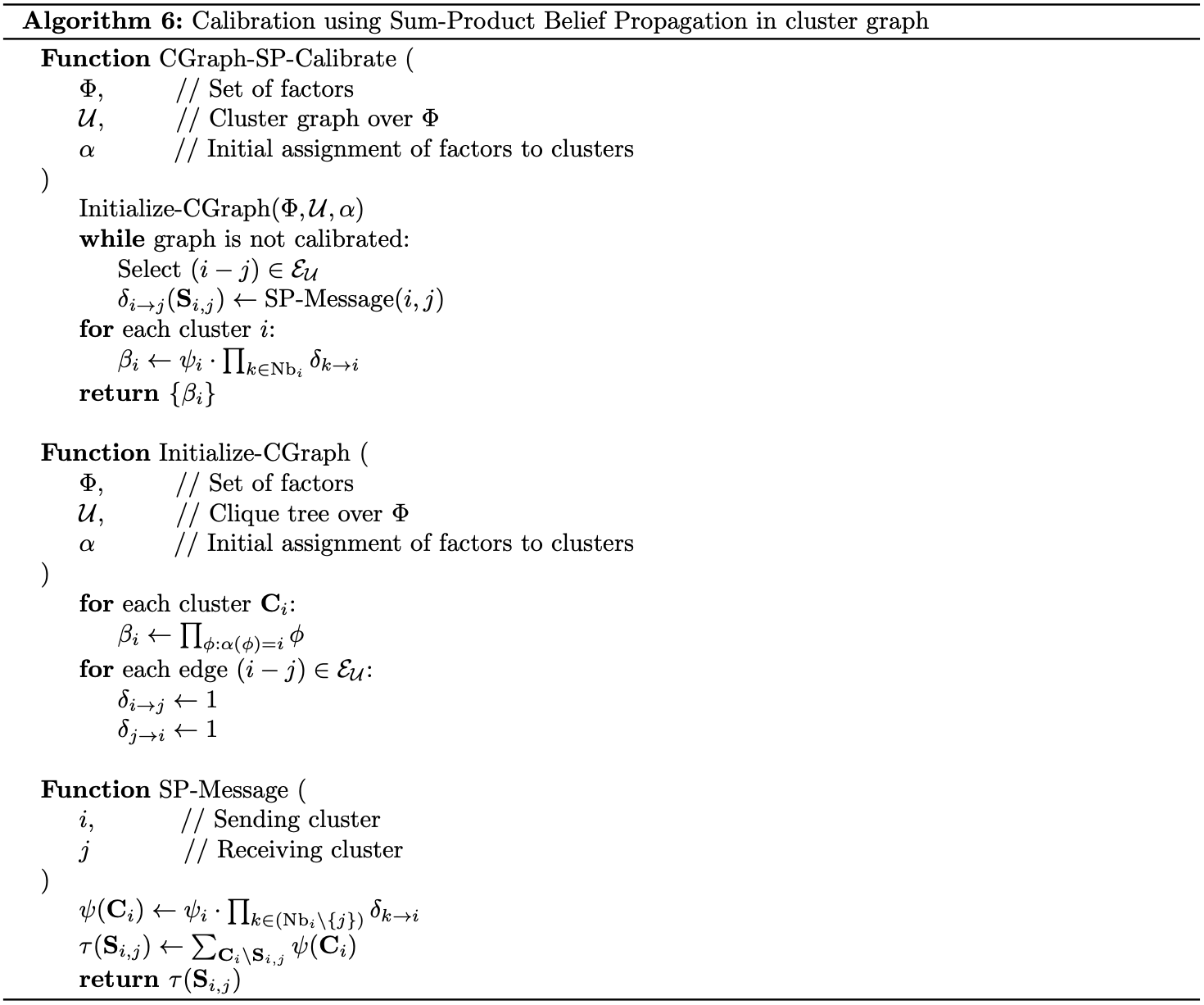
In this section, we consider approximation methods that use the same message propagation as in exact inference, but on a cluster graph, which might contain loops, rather than a clique tree.

Cluster-Graph Belief Propagation

Let $\mathbf{U}$ be a cluster graph. We say that $\mathbf{U}$ satisfies the running intersection property if whenever there is a variable $X$ such that $X\in\mathbf{C}_i$ and $\mathbf{C}_j$, then there is a single path between $\mathbf{C}_i$ and $\mathbf{C}_j$ for which $X\in\mathbf{S}_e$ for all edges $e$ in the path.

This property implies that all edges associated with $X$ form a tree that spans all the clusters that contain $X$.

Analogy to clique trees, in a cluster graph, we can also associate each cluster $\mathbf{C}_i$ with beliefs $\beta_i$. And in order to do the inference, it is necessary to perform beliefs calibration. We say that a cluster graph is calibrated if for each $(i-j)$ connecting the clusters $\mathbf{C}_i$ and $\mathbf{C}_j$, we have that¹ \begin{equation} \sum_{\mathbf{C}_i\backslash\mathbf{S}_{i,j}}\beta_i=\sum_{\mathbf{C}_j\backslash\mathbf{S}_{i,j}}\beta_j, \end{equation} which also means the two clusters agree on the marginal of variables in $\mathbf{S}_{i,j}$, as in clique trees.

Additionally, so as to clique trees, if a calibrated cluster graph satisfies the running intersection property, then the marginal of a variable $X$ in all the clusters containing it are identical.

When applying sum-product message passing algorithm on a cluster tree, specifically with a loopy cluster graph, we can not define whether a cluster is ready to transmit its message to its neighbor due to initially there is no cluster that has received any incoming messages. However, using the idea of belief propagation, which has been proved to be equivalent to sum-product, we can initialize all messages $\delta_{i\to j}=1$ (recalling that in clique tree belief propagation, we initialize $\mu_{i,j}=1$). Then, we can continue to use sum-product scheme for the cluster graph calibration. Similarly, we can also apply the belief-update message passing for cluster graphs. These algorithms are referred as variants of cluster-graph belief propagation class.

Properties of Cluster-Graph Belief Propagation

Properties of belief propagation procedure on clique trees can also extend to cluster graphs.

Reparameterization

Recall that belief propagation on clique trees maintains an invariant property, which let us show that the convergence point represent a reparameterization of the original distribution. This property can generalize to cluster graphs, resulting in the cluster graph invariant.

Theorem 18: Let $\mathcal{U}$ be a cluster graph over a set of factors $\Phi$. Consider the set of beliefs $\{\beta_i\}_{i\in\mathcal{V}_\mathcal{U}}$ and $\{\mu_{i,j}\}_{(i-j)\in\mathcal{E}_\mathcal{U}}$ at any iteration of $\text{CGraph-BU-Calibrate}$, then \begin{equation} \tilde{P}_\Phi(\mathcal{X})=\frac{\prod_{i\in\mathcal{V}_\mathcal{U}}\beta_i[\mathbf{C}_i]}{\prod_{(i-j)\in\mathcal{E}_\mathcal{U}}\mu_{i,j}[\mathbf{S}_{i,j}]} \end{equation}

Proof
We have \begin{align} \frac{\prod_{i\in\mathcal{V}_\mathcal{U}}\beta_i[\mathbf{C}_i]}{\prod_{(i-j)\in\mathcal{E}_\mathcal{U}}\mu_{i,j}[\mathbf{S}_{i,j}]}&=\frac{\prod_{i\in\mathcal{V}_\mathcal{U}}\left(\psi_i\prod_{j\in\text{Nb}_i}\delta_{j\to i}[\mathbf{S}_{i,j}]\right)}{\prod_{(i-j)\in\mathcal{E}_\mathcal{U}}\delta_{i\to j}[\mathbf{S}_{i,j}]\delta_{j\to i}[\mathbf{S}_{i,j}]} \\ &=\frac{\Big(\prod_{i\in\mathcal{V}_\mathcal{U}}\psi_i[\mathbf{C}_i]\Big)\left(\prod_{(i-j)\in\mathcal{E}_\mathcal{U}}\delta_{i\to j}[\mathbf{S}_{i,j}]\delta_{j\to i}[\mathbf{S}_{i,j}]\right)}{\prod_{(i-j)\in\mathcal{E}_\mathcal{U}}\delta_{i\to j}[\mathbf{S}_{i,j}]\delta_{j\to i}[\mathbf{S}_{i,j}]} \\ &=\prod_{i\in\mathcal{V}_\mathcal{U}}\psi_i[\mathbf{C}_i]=\prod_{\phi\in\Phi}\phi(\mathbf{U}_\phi)=\tilde{P}_\Phi(\mathcal{X}) \end{align}

Tree Consistency

Convergence of Cluster-Graph Belief Propagation

We will examine the convergence of belief propagation (BP) on a variant of its called synchronous BP, which performs all of the message updates simultaneously.

Consider the update step that takes all of the messages $\boldsymbol{\delta}^t$ at a particular iteration $t$ and produces new set of messages $\boldsymbol{\delta}^{t+1}$ for the next step. Let $\Delta$ be the space of all of possible messages in the cluster graph, then the belief-propagation update operator can be seen as a function $G_\text{BP}:\Delta\mapsto\Delta$. Consider the sum-product message update \begin{equation} \delta_{i\to j}’\propto\sum_{\mathbf{C}_i\backslash\mathbf{S}_{i,j}}\psi_i\cdot\prod_{k\in(\text{Nb}_i\backslash\{j\})}\delta_{k\to i}, \end{equation} where we normalize each message to sum to $1$². We continue to define the BP operator as the functions that simultaneously takes one set of messages and produces a new one \begin{equation} G_\text{BP}(\{\delta_{i\to j}\})=\{\delta_{i\to j}’\} \end{equation} Thus, the problem remains to examining the convergence property of $G_\text{BP}$, which can handled with the concept of Contraction Mapping and Banach’s Fixed-point theorem.

Constructing Cluster Graph

Unlike performing exact inference on clique trees, in cluster graph approximations, different graphs might lead to different results.

Pairwise Markov Networks

Bethe Cluster Graph

Structured Variational Approximations

In structured variational approximation, we want to solve the problem \begin{align} &\text{Find}&& Q\in\mathcal{Q} \\ &\text{maximizing}&& F[\tilde{P}_\Phi,Q]\label{eq:sva.1} \end{align} where $\mathcal{Q}$ is a given family of distributions.

The Mean Field Approximation

The Mean Field Energy

The mean field algorithm finds the distribution $Q$, which is closest to $P_\Phi$ in terms of the relative entropy $D_\text{KL}(Q\Vert P_\Phi)$ within the class of distributions $\mathcal{Q}$ representable as product of independent marginals \begin{equation} Q(\mathcal{X})=\prod_i Q(X_i) \end{equation} Hence, the energy functional can be rewritten as \begin{align} F[\tilde{P}_\Phi,Q]&=\sum_{\phi\in\Phi}\mathbb{E}_Q\big[\log\phi\big]+H_Q(\mathcal{X}) \\ &=\sum_{\phi\in\Phi}\mathbb{E}_{\mathbf{U}_\phi\sim Q}\big[\log\phi\big]+\mathbb{E}_Q\big[-\log Q(\mathcal{X})\big] \\ &=\sum_{\phi\in\Phi}\sum_{\mathbf{u}_\phi}Q(\mathbf{u}_\phi)\log\phi(\mathbf{u}_\phi)+\mathbb{E}_Q\Big[-\sum_i\log Q(X_i)\Big] \\ &=\sum_{\phi\in\Phi}\sum_{\mathbf{u}_\phi}\left(\prod_{X_i\in\mathbf{U}_i}Q(x_i)\right)\log\phi(\mathbf{u}_i)+\sum_i\mathbb{E}_Q\big[-\log Q(X_i)\big] \\ &=\sum_{\phi\in\Phi}\sum_{\mathbf{u}_\phi}\left(\prod_{X_i\in\mathbf{U}_i}Q(x_i)\right)\log\phi(\mathbf{u}_i)+\sum_i H_Q(X_i)\label{eq:mfe.1} \end{align}

Fixed-point Characterization

Our problem then is to optimize the mean field energy. \begin{align} &\text{Find}&&\{Q(X_i)\}\label{eq:fpc.1} \\ &\text{maximizing}&& F[\tilde{P},Q]\nonumber \\ &\text{s.t.}&& Q(\mathcal{X})=\prod_i Q(X_i)\nonumber \\ &&&\sum_{x_i}Q(x_i)=1,\hspace{1cm}\forall i\nonumber \end{align} Unlike the cluster-graph belief propagation and the expectation propagation algorithms, in Mean Field algorithm, we are not approximating the objective, but the optimization space by selecting a space of distributions $\mathcal{Q}$ that generally does not contain our original distribution $P_\Phi$.

The structure of $Q$ as a factored distribution gives us the following fixed-point equations that characterize the stationary points of the optimization problem \eqref{eq:fpc.1}.

Theorem 19: The distribution $Q(X_i)$ is a local maximum of \eqref{eq:fpc.1} given $\{Q(X_j)\}_{j\neq i}$ iff \begin{equation} Q(x_i)=\frac{1}{Z_i}\exp\left(\sum_{\phi\in\Phi}\mathbb{E}_{\mathcal{X}\sim Q}\big[\log\phi\vert x_i\big]\right),\label{eq:fpc.2} \end{equation} where $Z_i$ is a local normalizing constant.

Proof
Using the result \eqref{eq:mfe.1}, we have that the Lagrangian of the optimization problem \eqref{eq:fpc.1} is \begin{align} \mathcal{L}=-\sum_{\phi\in\Phi}\mathbb{E}_{\mathbf{U}_\phi\sim Q}\big[\log\phi\big]-\sum_i H_Q(X_i)+\sum_i\lambda_i\left(\sum_{x_i}Q(x_i)-1\right) \end{align} Differentiating the Lagrangian w.r.t $Q(x_i)$ gives us \begin{align} \frac{\partial\mathcal{L}}{\partial Q(x_i)}&=\frac{\partial}{\partial Q(x_i)}\left[-\sum_{\phi\in\Phi}\mathbb{E}_{\mathbf{U}_\phi\sim Q}\big[\log\phi\big]-H_Q(X_i)-\lambda_i\left(\sum_{x_i}Q(x_i)-1\right)\right] \\ &=-\sum_{\phi\in\Phi}\frac{\partial}{\partial Q(x_i)}\mathbb{E}_{\mathbf{U}_\phi\sim Q}\big[\log\phi\big]+\frac{\partial}{\partial Q(x_i)}Q(x_i)\log Q(x_i)-\lambda_i \\ &=-\sum_{\phi\in\Phi}\mathbb{E}_{\mathbf{U}_\Phi\sim Q}\big[\log\phi\vert x_i\big]+\log Q(x_i)+1-\lambda_i \\ &=-\sum_{\phi\in\Phi}\mathbb{E}_{\mathcal{X}\sim Q}\big[\log\phi\vert x_i\big]+\log Q(x_i)+1-\lambda_i \end{align} Setting this derivative to zero, we have that \begin{equation} Q(x_i)=\exp(\lambda_i-1)\exp\left(\sum_{\phi\in\Phi}\mathbb{E}_{\mathcal{X}\sim Q}\big[\log\phi\vert x_i\big]\right) \end{equation} From this result, it follows that

Proposition 20: The distribution $Q$ is a stationary point of \eqref{eq:fpc.1} iff for each $X_i$, equation \eqref{eq:fpc.2} holds.

Corollary 21: In the mean field approximation, $Q(X_i)$ is locally optimal only if \begin{equation} Q(x_i)=\frac{1}{Z_i}\exp\Big(\mathbb{E}_{\mathbf{X}_{-i}\sim Q}\Big[\log P_\Phi(x_i\vert\mathbf{X}_{-i})\Big]\Big), \end{equation} where we define $\mathbf{X}_{-i}\doteq\mathcal{X}\backslash\{X_i\}$ and where $Z_i$ is a normalizing constant.

Proof
Recall that $\tilde{P}_\Phi(\mathcal{X})=\prod_{\phi\in\Phi}\phi$. Thus by the linearity of expectation we have \begin{align} \sum_{\phi\in\Phi}\mathbb{E}_{\mathcal{X}\sim Q}\big[\log\phi\big\vert x_i\big]&=\mathbb{E}_{\mathcal{X}\sim Q}\left[\sum_{\phi\in\Phi}\log\phi\Big\vert x_i\right] \\ &=\mathbb{E}_{\mathcal{X}\sim Q}\left[\log\left(\prod_{\phi\in\Phi}\phi\Big\vert x_i\right)\right] \\ &=\mathbb{E}_{\mathcal{X}\sim Q}\big[\log\tilde{P}_\Phi(\mathcal{X})\big\vert x_i\big] \\ &=\mathbb{E}_{\mathcal{X}\sim Q}\big[\log\tilde{P}_\Phi(\mathbf{X}_{-i},X_i)\big\vert x_i\big] \\ &=\mathbb{E}_{\mathbf{X}_{-i}\sim Q}\big[\log\tilde{P}_\Phi(\mathbf{X}_{-i},x_i)\big] \\ &=\mathbb{E}_{\mathbf{X}_{-i}\sim Q}\big[\log\big(Z P_\Phi(\mathbf{X}_{-i},x_i)\big)\big] \\ &=\mathbb{E}_{\mathbf{X}_{-i}\sim Q}\big[\log\big(Z P_\Phi(\mathbf{X}_{-i})P_\Phi(x_i\vert\mathbf{X}_{-i})\big)\big] \\ &=\mathbb{E}_{\mathbf{X}_{-i}\sim Q}\big[\log P_\Phi(x_i\vert\mathbf{X}_{-i})\big]+\mathbb{E}_{\mathbf{X}_{-i}\sim Q}\big[\log\big(Z P_\Phi(\mathbf{X}_{-i})\big)\big] \end{align} Hence, by \eqref{eq:fpc.2}, we obtain \begin{align} Q(x_i)=\frac{1}{Z_i}\exp\Big(\mathbb{E}_{\mathbf{X}_{-i}\sim Q}\big[\log P_\Phi(x_i\vert\mathbf{X}_{-i})\big]\Big)\exp\Big(\mathbb{E}_{\mathbf{X}_{-i}\sim Q}\big[\log\big(Z P_\Phi(\mathbf{X}_{-i})\big)\big]\Big) \end{align} Notice that the latter exponential is a constant w.r.t $x_i$ and when multiplying a factor with a constant factor, it does not change the distribution $Q$, i.e. the constant will be absorbed into the normalizing function.

The Mean Field Algorithm

Corollary 22: In the mean field approximation, $Q(X_i)$ is locally optimal only if \begin{equation} Q(x_i)=\frac{1}{Z_i}\exp\left(\sum_{\phi:X_i\in\text{Scope}(\phi)}\mathbb{E}_{(\mathbf{U}_\phi\backslash\{X_i\})\sim Q}\big[\log\phi(\mathbf{U}_\phi,x_i)\big]\right) \end{equation} In other words, $Q(X_i)$ has to be consistent with the expectation of the potentials in which it appears. We thus obtain the following algorithm

Variational Inference

References

[1] Daphne Koller, Nir Friedman. Probabilistic Graphical Models. The MIT Press.

Footnotes