Notes on using linear models in regression and classification.
Preliminaries
Independence, basis in vector space
Linear independence
The sequence of vectors $\mathbf{x}_1,\ldots,\mathbf{x}_n$ is said to be linearly independent (or independent) if \begin{equation} c_1\mathbf{x}_1+\ldots+c_n\mathbf{x}_n=\mathbf{0} \end{equation} only when $c_1,\ldots,c_n$ are all zero.
Considering those $n$ vectors $\mathbf{x}_1,\ldots,\mathbf{x}_n$ as $n$ columns of a matrix $\mathbf{A}$ \begin{equation} \mathbf{A}=\left[\begin{matrix}\vert&&\vert \\ \mathbf{x}_1 & \ldots & \mathbf{x}_n \\ \vert&&\vert\end{matrix}\right] \end{equation} we have that the columns of $\mathbf{A}$ are independent when \begin{equation} \mathbf{A}\mathbf{x}=\mathbf{0}\hspace{0.5cm}\Leftrightarrow\hspace{0.5cm}\mathbf{x}=\mathbf{0}, \end{equation} or in other words, the rank of $\mathbf{A}$ is equal to the number of columns of $\mathbf{A}$.
Basis of a vector space
We say that vectors $\mathbf{v}_1,\ldots,\mathbf{v}_k$ span a space $S$ when the space consists of all combinations of those vectors. Or in other words, any vector $\mathbf{u}\in S$ can be displayed as linear combination of $\mathbf{v}_i$.
In this case, $S$ is the smallest space containing those vectors.
A basis for a vector space $S$ is a sequence of vectors $\mathbf{v}_1,\ldots,\mathbf{v}_d$ having two properties:
- $\mathbf{v}_1,\ldots,\mathbf{v}_d$ are independent
- $\mathbf{v}_1,\ldots,\mathbf{v}_d$ span $S$
With that definition of a basis $\mathbf{v}_1,\dots,\mathbf{v}_d$ of $S$, for each vector $\mathbf{u}\in S$, there exists only one sequence $c_1,\ldots,c_d$ such that \begin{equation} \mathbf{u}=c_1\mathbf{v}_1+\ldots+c_d\mathbf{v}_d \end{equation}
Lagrange Multipliers
Consider the problem of finding the maximum (or minimum) of $w=f(x_1,x_2,x_3)$ subject to a constraint relating $x_1,x_2$ and $x_3$ \begin{equation} g(x_1,x_2,x_3)=0 \end{equation} Apart from solving $x_3$ in terms of $x_1$ and $x_2$ in the constraint and substituting into the original function, which now becomes an unconstrained, here we can also solve this problem as a constrained one.
The idea is we are using the observation that the gradient vector $\nabla f(\mathbf{x})$ and $\nabla g(\mathbf{x})$ are parallel, because:
Suppose $f(\mathbf{x})$ has a local maximum at $\mathbf{x}^*$ on the constraint surface $g(\mathbf{x})=0$.
Let $\mathbf{r}(t)=\langle x_1(t),x_2(t),x_3(t)\rangle$ be a parameterized curve on the constraint surface such that and $\mathbf{r}(t)$ has \begin{equation} (x_1(0),x_2(0),x_3(0))^\text{T}=\mathbf{x} \end{equation} And also, let $h(t)=f(x_1(t),x_2(t),x_3(t))$, then it implies that $h$ has a maximum at $t=0$, which lets \begin{equation} h’(0)=0 \end{equation} Taking the derivative of $h$ w.r.t, we obtain \begin{equation} h’(t)=\nabla f(\mathbf{x})\big\vert_{\mathbf{r}(t)}\mathbf{r}’(t) \end{equation} Therefore, \begin{equation} \nabla f(\mathbf{x})\big\vert_{\mathbf{x}^*}\mathbf{r}’(0)=0, \end{equation} which implies that $\nabla f(\mathbf{x})$ is perpendicular to any curve in the constraint space that goes through $\mathbf{x}^*$. And since $\nabla g(\mathbf{x})$ perpendicular to the constraint surface $g(x)=0$, then $\nabla g(\mathbf{x})$ is also perpendicular to those curves. This implies that $\nabla f(\mathbf{x})$ is parallel to $\nabla g(\mathbf{x})$.
With this property, we can write $\nabla f(\mathbf{x})$ in terms of $\nabla g(\mathbf{x})$, as \begin{equation} \nabla f(\mathbf{x})=\lambda\nabla g(\mathbf{x}), \end{equation} where $\lambda\neq 0$ is a constant called Lagrange multiplier.
With this definition of Lagrange multiplier, we continue to define the Lagrangian function, given as \begin{equation} \mathcal{L}(\mathbf{x},\lambda)=f(\mathbf{x})+\lambda g(\mathbf{x}) \end{equation} Then letting the partial derivative of Lagrangian w.r.t $\lambda$ be zero gives us the constraint \begin{equation} 0=\frac{\partial \mathcal{L}(\mathbf{x},\lambda)}{\partial\lambda}=g(\mathbf{x}) \end{equation} With Lagrangian, in order to find the maximum of $f(\mathbf{x})$ that satisfies $g(\mathbf{x})=0$, we will instead be trying to solve \begin{equation} \max_\mathbf{x}\min_\lambda\mathcal{L}(\mathbf{x},\lambda), \end{equation} This can be solved by letting derivatives of the Lagrangian $\mathcal{L}$ w.r.t $x_i$ (i.e. components of $\mathbf{x}$) and $\lambda$ be zero \begin{equation} \frac{\partial\mathcal{L}}{\partial x_i}=0,\hspace{1cm}\frac{\partial\mathcal{L}}{\partial\lambda}=0 \end{equation} and solve for $x_i$ and $\lambda$.
Linear models for Regression
Regression refers to a problem of predicting the value of one or more continuous target variable $t$ given the value of a $D$-dimensional vector $\mathbf{x}$ of input variables.
Linear basis function models
The simplest linear model used for regression tasks is linear regression, which is defined as a linear combination of the input variables \begin{equation} y(\mathbf{x},\mathbf{w})=w_0+w_1x_1+\ldots+w_Dx_D, \end{equation} where $\mathbf{x}=(x_1,\ldots,x_D)^\text{T}$ is the input variables, while $w_i$’s are the parameters parameterizing the space of linear function mapping from the input space $\mathcal{X}$ of $\mathbf{x}$ to $\mathcal{Y}$.
With the idea of spanning a space by its basis vectors, we can generalize it to establishing a function space by linear combinations of simpler basis functions. Or in other words, we can extend the class of models by instead using a linear combination of fixed nonlinear functions of the input variables $\mathbf{x}$, as \begin{equation} y(\mathbf{x},\mathbf{w})=w_0+w_1\phi_1(\mathbf{x})+\ldots+w_{M-1}\phi_{M-1}(\mathbf{x})=w_0+\sum_{i=1}^{M-1}w_i\phi_i(\mathbf{x}),\label{eq:lbfm.1} \end{equation} where $\phi_i(\mathbf{x})$’s are called the basis functions; $w_0$ is called a bias parameter. By letting $w_0$ be a coefficient corresponding to a dummy basis function $\phi_0(\mathbf{x})=1$, \eqref{eq:lbfm.1} can be written in a more convenient way \begin{equation} y(\mathbf{x},\mathbf{w})=\sum_{i=0}^{M-1}w_i\phi_i(\mathbf{x})=\mathbf{w}^\text{T}\boldsymbol{\phi}(\mathbf{x}),\label{eq:lbfm.2} \end{equation} where $\mathbf{w}=(w_0,\ldots,w_{M-1})^\text{T}$ and $\boldsymbol{\phi}=(\phi_0,\ldots,\phi_{M-1})^\text{T}$, with $\phi_0(\cdot)=1$.
There are various choices of basis functions:
- Polynomial basis. Each basis function $\phi_i$ is a powers of a $1$-dimensional input $x$:
\begin{equation}
\phi_i(x)=x^i
\end{equation}
An example of polynomial basis functions is illustrated as below
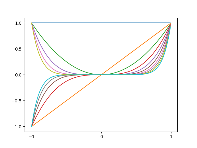
Figure 1: (based on figure from Bishop's book) Example of polynomial basis functions. The code can be found here - Gaussian basis function. Each basis function $\phi_i$ is a Gaussian function of a $1$-dimensional input $x$:
\begin{equation}
\phi_i(x)=\exp\left(-\frac{(x-\mu_i)^2}{2\sigma_i^2}\right)
\end{equation}
An example of Gaussian basis functions is illustrated as below
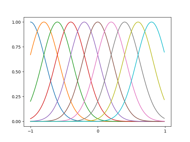
Figure 2: (based on figure from Bishop's book) Example of Gaussian basis functions. The code can be found here - Sigmoidal basis function. Each basis function $\phi_i$ is defined as
\begin{equation}
\phi_i(x)=\sigma\left(\frac{x-\mu_i}{\sigma_i}\right),
\end{equation}
where $\sigma(\cdot)$ is the logistic sigmoid function
\begin{equation}
\sigma(x)=\frac{1}{1+\exp(-x)}
\end{equation}
An example of sigmoidal basis functions is illustrated as below
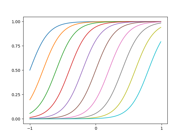
Figure 3: (based on figure from Bishop's book) Example of sigmoidal basis functions. The code can be found here
Least squares
Assume that the target variable $t$ and the inputs $\mathbf{x}$ is related via the equation \begin{equation} t=y(\mathbf{x},\mathbf{w})+\epsilon, \end{equation} where $\epsilon$ is an error term that captures random noise such that $\epsilon\sim\mathcal{N}(0,\sigma^2)$, which means the density of $\epsilon$ can be written as \begin{equation} p(\epsilon)=\frac{1}{\sqrt{2\pi}\sigma}\exp\left(-\frac{\epsilon^2}{2\sigma^2}\right), \end{equation} which implies that \begin{equation} p(t|\mathbf{x};\mathbf{w},\beta)=\sqrt{\frac{\beta}{2\pi}}\exp\left(-\frac{(t-y(\mathbf{x},\mathbf{w}))^2\beta}{2}\right),\label{eq:lsr.1} \end{equation} where $\beta=1/\sigma^2$ is the precision of $\epsilon$, or \begin{equation} t|\mathbf{x};\mathbf{w},\beta\sim\mathcal{N}(y(\mathbf{x},\mathbf{w}),\beta^{-1}) \end{equation} Consider a data set of inputs $\mathbf{X}=\{\mathbf{x}_1,\ldots,\mathbf{x}_N\}$ with corresponding target values $\mathbf{t}=(t_1,\ldots,t_N)^\text{T}$ and assume that these data points are drawn independently from the distribution above, we obtain the batch version of \eqref{eq:lsr.1}, called the likelihood function, given as \begin{align} L(\mathbf{w},\beta)=p(\mathbf{t}|\mathbf{X};\mathbf{w},\beta)&=\prod_{i=1}^{N}p(t_i|\mathbf{x}_i;\mathbf{w},\beta) \\ &=\prod_{i=1}^{N}\sqrt{\frac{\beta}{2\pi}}\exp\left(-\frac{(t_i-y(\mathbf{x}_i,\mathbf{w}))^2\beta}{2}\right)\label{eq:lsr.2} \end{align} By maximum likelihood, we will be looking for values of $\mathbf{w}$ and $\beta$ that maximize the likelihood. We do this by considering maximizing a simpler likelihood, called log likelihood, denoted as $\ell(\mathbf{w},\beta)$, defined as \begin{align} \ell(\mathbf{w},\beta)=\log{L(\mathbf{w},\beta)}&=\log\prod_{i=1}^{N}\sqrt{\frac{\beta}{2\pi}}\exp\left(-\frac{(t_i-y(\mathbf{x}_i,\mathbf{w}))^2\beta}{2}\right) \\ &=\sum_{i=1}^{N}\log\left[\sqrt{\frac{\beta}{2\pi}}\exp\left(-\frac{(t_i-y(\mathbf{x}_i,\mathbf{w}))^2\beta}{2}\right)\right] \\ &=\frac{N}{2}\log\beta-\frac{N}{2}\log(2\pi)-\sum_{i=1}^{N}\frac{(t_i-y(\mathbf{x}_i,\mathbf{w}))^2\beta}{2} \\ &=\frac{N}{2}\log\beta-\frac{N}{2}\log(2\pi)-\beta E_D(\mathbf{w})\label{eq:lsr.3}, \end{align} where $E_D(\mathbf{w})$ is the sum-of-squares error function, defined as \begin{equation} E_D(\mathbf{w})\doteq\frac{1}{2}\sum_{i=1}^{N}\left(t_i-y(\mathbf{x}_i,\mathbf{w})\right)^2\label{eq:lsr.4} \end{equation} Consider the gradient of \eqref{eq:lsr.3} w.r.t $\mathbf{w}$, we have \begin{align} \nabla_\mathbf{w}\ell(\mathbf{w},\beta)&=\nabla_\mathbf{w}\left[\frac{N}{2}\log\beta-\frac{N}{2}\log(2\pi)-\beta E_D(\mathbf{w})\right] \\ &\propto\nabla_\mathbf{w}\frac{1}{2}\sum_{i=1}^{N}\big(t_i-y(\mathbf{x}_i,\mathbf{w})\big)^2 \\ &=\nabla_\mathbf{w}\frac{1}{2}\sum_{i=1}^{N}\left(t_i-\mathbf{w}^\text{T}\boldsymbol{\phi}\big(\mathbf{x}_i\right)\big)^2 \\ &=\sum_{i=1}^{N}(t_i-\mathbf{w}^\text{T}\boldsymbol{\phi}(\mathbf{x}_i))\boldsymbol{\phi}(\mathbf{x}_i)^\text{T} \end{align} By gradient descent, letting this gradient to zero gives us \begin{equation} \sum_{i=1}^{N}t_i\boldsymbol{\phi}(\mathbf{x}_i)^\text{T}-\mathbf{w}^\text{T}\sum_{i=1}^{N}\boldsymbol{\phi}(\mathbf{x}_i)\boldsymbol{\phi}(\mathbf{x}_i)^\text{T}=0, \end{equation} which implies that \begin{equation} \mathbf{w}_\text{ML}=\left(\boldsymbol{\Phi}^\text{T}\boldsymbol{\Phi}\right)^{-1}\boldsymbol{\Phi}^\text{T}\mathbf{t},\label{eq:lsr.5} \end{equation} which is known as the normal equations for the least squares problem. In \eqref{eq:lsr.5}, $\boldsymbol{\Phi}\in\mathbb{R}^{N\times M}$ is called the design matrix, whose elements are given by $\boldsymbol{\Phi}_{ij}=\phi_j(\mathbf{x}_i)$ \begin{equation} \boldsymbol{\Phi}=\left[\begin{matrix}-\hspace{0.1cm}\boldsymbol{\phi}(\mathbf{x}_1)^\text{T}\hspace{0.1cm}- \\ \hspace{0.1cm}\vdots\hspace{0.1cm} \\ -\hspace{0.1cm}\boldsymbol{\phi}(\mathbf{x}_N)^\text{T}\hspace{0.1cm}-\end{matrix}\right]=\left[\begin{matrix}\phi_0(\mathbf{x}_1)&\ldots&\phi_{M-1}(\mathbf{x}_1) \\ \vdots&\ddots&\vdots \\ \phi_0(\mathbf{x}_N)&\ldots&\phi_{M-1}(\mathbf{x}_N)\end{matrix}\right], \end{equation} and the quantity \begin{equation} \boldsymbol{\Phi}^\dagger\doteq\left(\boldsymbol{\Phi}^\text{T}\boldsymbol{\Phi}\right)^{-1}\boldsymbol{\Phi}^\text{T} \end{equation} is called the Moore-Penrose pseudoinverse of the matrix $\boldsymbol{\Phi}$.
On the other hand, consider the gradient of \eqref{eq:lsr.3} w.r.t $\beta$ and set it equal to zero, we obtain \begin{equation} \beta=\frac{N}{\sum_{i=1}^{N}\big(t_i-\mathbf{w}_\text{ML}^\text{T}\boldsymbol{\phi}(\mathbf{x}_i)\big)^2} \end{equation}
Geometrical interpretation of least squares
As mentioned before, we have applied the idea of spanning a vector space by its basis vectors when constructing basis functions.
In particular, consider an $N$-dimensional space whose axes are given by $t_i$, which implies that \begin{equation} \mathbf{t}=(t_1,\ldots,t_N)^\text{T} \end{equation} is a vector contained in the space.
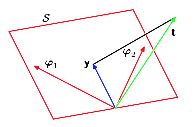
Each basis function $\phi_j(\mathbf{x}_i)$, evaluated at the $N$ data points, then can also be presented as a vector in the same space, denoted by $\boldsymbol{\varphi}_j$, as illustrated in Figure 4 above. Therefore, the design matrix $\boldsymbol{\Phi}$ can be represented as \begin{equation} \boldsymbol{\Phi}=\left[\begin{matrix}-\hspace{0.1cm}\boldsymbol{\phi}(\mathbf{x}_1)\hspace{0.1cm}- \\ \hspace{0.1cm}\vdots\hspace{0.1cm} \\ -\hspace{0.1cm}\boldsymbol{\phi}(\mathbf{x}_N)\hspace{0.1cm}-\end{matrix}\right]=\left[\begin{matrix}\vert&&\vert \\ \boldsymbol{\varphi}_{0}&\ldots&\boldsymbol{\varphi}_{M-1} \\ \vert&&\vert\end{matrix}\right] \end{equation} When the number $M$ of basis functions is smaller than the number $N$ of data points, the $M$ vectors $\phi_j(\mathbf{x}_i)$ will span a linear subspace $\mathcal{S}$ of $M$ dimensions.
We define $\mathbf{y}$ to be an $N$-dimensional vector whose the $i$-th element is given by $y(\mathbf{x}_i,\mathbf{w})$ \begin{equation} \mathbf{y}=\big(y(\mathbf{x}_1,\mathbf{w}),\ldots,y(\mathbf{x}_N,\mathbf{w})\big)^\text{T} \end{equation} Since $\mathbf{y}$ is a linear combination of $\boldsymbol{\varphi}_i$, then $\mathbf{y}\in\mathcal{S}$. Then the sum-of-squares error \eqref{eq:lsr.4} is exactly (with a factor of $1/2$) the squared Euclidean distance between $\mathbf{y}$ and $\mathbf{t}$. Therefore, the least square solution to $\mathbf{w}$ is the one that makes $\mathbf{y}$ closest to $\mathbf{t}$.
This solution corresponds to the orthogonal projection of $t$ onto the subspace $S$ spanned by $\boldsymbol{\varphi}_i$, because we have that \begin{align} \mathbf{y}^\text{T}(\mathbf{t}-\mathbf{y})&=\left(\boldsymbol{\Phi}\mathbf{w}_\text{ML}\right)^\text{T}\left(\mathbf{t}-\boldsymbol{\Phi}\mathbf{w}_\text{ML}\right) \\ &=\left(\boldsymbol{\Phi}\left(\boldsymbol{\Phi}^\text{T}\boldsymbol{\Phi}\right)^{-1}\boldsymbol{\Phi}\mathbf{t}\right)^\text{T}\left(\mathbf{t}-\boldsymbol{\Phi}\left(\boldsymbol{\Phi}^\text{T}\boldsymbol{\Phi}\right)^{-1}\boldsymbol{\Phi}\mathbf{t}\right) \\ &=\mathbf{t}^\text{T}\boldsymbol{\Phi}\left(\left(\boldsymbol{\Phi}^\text{T}\boldsymbol{\Phi}\right)^{-1}\right)^\text{T}\boldsymbol{\Phi}^\text{T}\mathbf{t}-\mathbf{t}^\text{T}\boldsymbol{\Phi}\left(\left(\boldsymbol{\Phi}^\text{T}\boldsymbol{\Phi}\right)^{-1}\right)^\text{T}\boldsymbol{\Phi}^\text{T}\boldsymbol{\Phi}\left(\boldsymbol{\Phi}^\text{T}\boldsymbol{\Phi}\right)^{-1}\boldsymbol{\Phi}\mathbf{t} \\ &=\mathbf{t}^\text{T}\boldsymbol{\Phi}\left(\left(\boldsymbol{\Phi}^\text{T}\boldsymbol{\Phi}\right)^{-1}\right)^\text{T}\boldsymbol{\Phi}^\text{T}\mathbf{t}-\mathbf{t}^\text{T}\boldsymbol{\Phi}\left(\left(\boldsymbol{\Phi}^\text{T}\boldsymbol{\Phi}\right)^{-1}\right)^\text{T}\boldsymbol{\Phi}^\text{T}\mathbf{t} \\ &=0, \end{align}
The LMS algorithm
The least-means-squares, or LMS algorithm for the sum-of-squares error \eqref{eq:lsr.4}, which start with some initial vector $\mathbf{w}_0$ of $\mathbf{w}$, and repeatedly perform the update \begin{equation} \mathbf{w}_{t+1}=\mathbf{w}_t+\eta(t_n-\mathbf{w}_t^\text{T}\boldsymbol{\phi}_n)\boldsymbol{\phi}_n, \end{equation} where $\boldsymbol{\phi}_n$ denotes $\boldsymbol{\phi}(\mathbf{x}_n)$, and $\eta$ is called the learning rate which controls the update amount.
Regularized least squares
To control over-fitting, in the error function \eqref{eq:lsr.4}, we add an regularization term, which makes the total error function to be minimized take the form \begin{equation} E_D(\mathbf{w})+\lambda E_W(\mathbf{w}),\label{eq:rls.1} \end{equation} where $\lambda$ is the regularization coefficient that controls the relative importance of the data-dependent error $E_D(\mathbf{w})$ and the regularization term $E_W(\mathbf{w})$. One simple possible form of regularizer is given as \begin{equation} E_W(\mathbf{w})=\frac{1}{2}\mathbf{w}^\text{T}\mathbf{w} \end{equation} The total error function \eqref{eq:rls.1} then can be written as \begin{equation} E_D(\mathbf{w})+E_W(\mathbf{w})=\frac{1}{2}\sum_{i=1}^{N}\big(t_i-\mathbf{w}^\text{T}\boldsymbol{\phi}(\mathbf{x}_i)\big)^2+\frac{\lambda}{2}\mathbf{w}^\text{T}\mathbf{w}\label{eq:rls.2} \end{equation} Setting the gradient of this error to zero and solving for $\mathbf{w}$, we have the solution \begin{equation} \mathbf{w}= (\lambda\mathbf{I}+\boldsymbol{\Phi}^\text{T}\boldsymbol{\Phi})^{-1}\boldsymbol{\Phi}^\text{T}\mathbf{t}\label{eq:rls.3} \end{equation} This particular choice of regularizer is called weight decay because it encourages weight values to decay towards zero in sequential learning.
Another choice of regularizer which is more general lets the regularized error have the form \begin{equation} E_D(\mathbf{w})+E_W(\mathbf{w})=\frac{1}{2}\sum_{i=1}^{N}\big(t_i-\mathbf{w}^\text{T}\boldsymbol{\phi}(\mathbf{x}_i)\big)^2+\frac{\lambda}{2}\sum_{j=1}^{M}\vert w_j\vert^q, \end{equation} where $q=2$ corresponds to the regularizer \eqref{eq:rls.2}.
Multiple outputs
When the target of our model is instead in multiple-dimensional form, denoted as $\mathbf{t}$, we can generalize our model to be \begin{equation} \mathbf{y}(\mathbf{x},\mathbf{w})=\mathbf{W}^\text{T}\boldsymbol{\phi}(\mathbf{x}), \end{equation} where $\mathbf{y}\in\mathbb{R}^K, \mathbf{W}\in\mathbb{R}^{M\times K}$ is the matrix of parameters, $\boldsymbol{\phi}\in\mathbb{R}^M$ with $\phi_i(\mathbf{x})$ as the $i$-th element, and with $\phi_0(\mathbf{x})=1$.
With this generalization, \eqref{eq:lsr.1} can be also be rewritten as \begin{equation} p(\mathbf{t}|\mathbf{x};\mathbf{W},\beta)=\sqrt{\frac{\beta}{2\pi\vert\mathbf{I}\vert}}\exp\left[-\frac{1}{2}\left(\mathbf{t}-\mathbf{W}^\text{T}\boldsymbol{\phi}\left(\mathbf{x}\right)\right)^\text{T}\left(\mathbf{t}-\mathbf{W}^\text{T}\boldsymbol{\phi}\left(\mathbf{x}\right)\right)\beta\mathbf{I}^{-1}\right], \end{equation} or in other words \begin{equation} \mathbf{t}|\mathbf{x};\mathbf{W},\beta\sim\mathcal{N}(\mathbf{W}^\text{T}\boldsymbol{\phi}(\mathbf{x}),\beta^{-1}\mathbf{I}) \end{equation} With a data set of inputs $\mathbf{X}=\{\mathbf{x}_1,\ldots,\mathbf{x}_N\}$, our target values can also be vectorized into $\mathbf{T}\in\mathbb{R}^{N\times K}$ given as \begin{equation} \mathbf{T}=\left[\begin{matrix}-\hspace{0.1cm}\mathbf{t}_1^\text{T}\hspace{0.1cm}- \\ \vdots \\ -\hspace{0.1cm}\mathbf{t}_N^\text{T}\hspace{0.1cm}-\end{matrix}\right], \end{equation} and likewise with the input matrix $\mathbf{X}$ vectorized from input vectors $\mathbf{x}_1,\ldots,\mathbf{x}_N$. With these definitions, the multi-dimensional likelihood can be defined as \begin{align} L(\mathbf{W},\beta)&=p(\mathbf{T}|\mathbf{X};\mathbf{W},\beta) \\ &=\prod_{i=1}^{N}p(\mathbf{t}_i|\mathbf{x}_i;\mathbf{W},\beta) \\ &=\prod_{i=1}^{N}\sqrt{\frac{\beta}{2\pi}}\exp\left[-\frac{\beta}{2}\big(\mathbf{t}_i-\mathbf{W}^\text{T}\boldsymbol{\phi}(\mathbf{x}_i)\big)^\text{T}\big(\mathbf{t}_i-\mathbf{W}^\text{T}\boldsymbol{\phi}(\mathbf{x}_i)\big)\right] \end{align} And thus the log likelihood now becomes \begin{align} \ell(\mathbf{W},\beta)&=\log L(\mathbf{W},\beta) \\ &=\log\prod_{i=1}^{N}\sqrt{\frac{\beta}{2\pi}}\exp\left[-\frac{\beta}{2}\big(\mathbf{t}_i-\mathbf{W}^\text{T}\boldsymbol{\phi}(\mathbf{x}_i)\big)^\text{T}\big(\mathbf{t}_i-\mathbf{W}^\text{T}\boldsymbol{\phi}(\mathbf{x}_i)\big)\right] \\ &=\sum_{i=1}^{N}\log\sqrt{\frac{\beta}{2\pi}}\exp\left[-\frac{\beta}{2}\big(\mathbf{t}_i-\mathbf{W}^\text{T}\boldsymbol{\phi}(\mathbf{x}_i)\big)^\text{T}\big(\mathbf{t}_i-\mathbf{W}^\text{T}\boldsymbol{\phi}(\mathbf{x}_i)\big)\right] \\ &=\frac{N}{2}\log\frac{\beta}{2\pi}-\frac{\beta}{2}\sum_{i=1}^{N}\big(\mathbf{t}_i-\mathbf{W}^\text{T}\boldsymbol{\phi}(\mathbf{x}_i)\big)^\text{T}\big(\mathbf{t}_i-\mathbf{W}^\text{T}\boldsymbol{\phi}(\mathbf{x}_i)\big) \end{align} Taking the gradient of the log likelihood w.r.t $\mathbf{W}$, setting it to zero and solving for $\mathbf{W}$ gives us \begin{equation} \mathbf{W}_\text{ML}=(\boldsymbol{\Phi}^\text{T}\boldsymbol{\Phi})^{-1}\boldsymbol{\Phi}^\text{T}\mathbf{T} \end{equation}
Bayesian linear regression
Parameter distribution
Consider the noise precision parameter $\beta$ as a constant. From the equation \eqref{eq:lsr.2}, we see that the likelihood function $L(\mathbf{w})=p(\mathbf{t}\vert\mathbf{w})$ takes the form of an exponential of a quadratic form in $\mathbf{w}$. Thus, if we choose the prior $p(\mathbf{w})$ as a Gaussian, the corresponding posterior will also become a Gaussian due to being computed as a product of two exponentials of quadratic forms of $\mathbf{w}$. This makes the prior be a conjugate distribution for the likelihood function, and hence be given by \begin{equation} p(\mathbf{w})=\mathcal{N}(\mathbf{w}\vert\mathbf{m}_0,\mathbf{S}_0), \end{equation} where $\mathbf{m}_0$ is the mean vector and $\mathbf{S}_0$ is the covariance matrix.
By the result, we have that the corresponding posterior distribution $p(\mathbf{w}\vert\mathbf{t})$, which is a conditional Gaussian distribution, is given by \begin{equation} p(\mathbf{w}\vert\mathbf{t})=\mathcal{N}(\mathbf{w}\vert\mathbf{m}_N,\mathbf{S}_N),\label{eq:pd.1} \end{equation} where the mean $\mathbf{m}_N$ and the precision matrix $\mathbf{S}_N^{-1}$ are defined as \begin{align} \mathbf{m}_N&=\mathbf{S}_N(\mathbf{S}_0^{-1}\mathbf{m}_0+\beta\boldsymbol{\Phi}^\text{T}\mathbf{t}), \\ \mathbf{S}_N^{-1}&=\mathbf{S}_0^{-1}+\beta\boldsymbol{\Phi}^\text{T}\boldsymbol{\Phi} \end{align} Therefore, by MAP, we have \begin{align} \mathbf{w}_\text{MAP}&=\underset{\mathbf{w}}{\text{argmax}}\hspace{0.1cm}\exp\Big[-\frac{1}{2}(\mathbf{w}-\mathbf{m}_N)^\text{T}\mathbf{S}_N^{-1}(\mathbf{w}-\mathbf{m}_N)\Big] \\ &=\underset{\mathbf{w}}{\text{argmin}}\hspace{0.1cm}(\mathbf{w}-\mathbf{m}_N)^\text{T}\mathbf{S}_N^{-1}(\mathbf{w}-\mathbf{m}_N) \end{align} By this property of the covariance matrix, we have that the precision matrix $\mathbf{S}_N^{-1}$ and the covariance matrix $\mathbf{S}_N$ have the same set of eigenvalues, which are non-negative due to the fact that $\mathbf{S}_N$ is positive semi-definite. This also means that $\mathbf{S}_N$ is positive semi-definite, and thus \begin{equation} (\mathbf{w}-\mathbf{m}_N)^\text{T}\mathbf{S}_N^{-1}(\mathbf{w}-\mathbf{m}_N)\geq0 \end{equation} Therefore, the maximum posterior weight vector is also the mean vector \begin{equation} \mathbf{w}_\text{MAP}=\mathbf{m}_N\label{eq:pd.2} \end{equation} Consider an infinite broad prior $\mathbf{S}_0=\alpha^{-1}\mathbf{I}$ with $\alpha\to 0$, in this case the mean $\mathbf{m}_N$ reduces to the maximum likelihood value $\mathbf{w}_\text{ML}$ given by \eqref{eq:lsr.5}. And if $N=0$, then the posterior distribution reverts to the prior.
Furthermore, consider an additional data point $(\mathbf{x}_{N+1},t_{N+1})$, the posterior given in \eqref{eq:pd.1} can be regarded as the prior distribution for that data point. If the model is given as \eqref{eq:lsr.1}, the likelihood function of the newly added data point is then given in form \begin{equation} p(t_{N+1}\vert\mathbf{x}_{N+1},\mathbf{w})=\left(\frac{\beta}{2\pi}\right)^{1/2}\exp\left(-\frac{(t_{N+1}-\mathbf{w}^\text{T}\boldsymbol{\phi}_{N+1})\beta}{2}\right), \end{equation} where $\boldsymbol{\phi}_{N+1}=\boldsymbol{\phi}(\mathbf{x}_{N+1})$. Therefore, the posterior distribution of the data point $(\mathbf{x}_{N+1},t_{N+1})$ can be computed as \begin{align} &\hspace{0.7cm}p(\mathbf{w}\vert t_{N+1},\mathbf{x}_{N+1},\mathbf{t}) \\ &\propto p(t_{N+1}\vert\mathbf{x}_{N+1},\mathbf{w})p(\mathbf{w}\vert\mathbf{t}) \\ &=\exp\Big[-\frac{1}{2}(\mathbf{w}-\mathbf{m}_N)^\text{T}\mathbf{S}_N^{-1}(\mathbf{w}-\mathbf{m}_N)-\frac{1}{2}(t_{N+1}-\mathbf{w}^\text{T}\boldsymbol{\phi}_{N+1})^2\beta\Big] \\ &=\exp\Big[-\frac{1}{2}\big(\mathbf{w}^\text{T}\mathbf{S}_N^{-1}\mathbf{w}+\beta\mathbf{w}^\text{T}\boldsymbol{\phi}_{N+1}\boldsymbol{\phi}_{N+1}^\text{T}\mathbf{w}\big)+\mathbf{w}^\text{T}\big(\mathbf{S}_N^{-1}\mathbf{m}_N+t_{N+1}\beta\boldsymbol{\phi}_{N+1}\big)+c\Big] \\ &=\exp\Big[-\frac{1}{2}\mathbf{w}^\text{T}\big(\mathbf{S}_N^{-1}+\beta\boldsymbol{\phi}_{N+1}\boldsymbol{\phi}_{N+1}^\text{T}\big)\mathbf{w}+\mathbf{w}^\text{T}\big(\mathbf{S}_N^{-1}\mathbf{m}_N+t_{N+1}\beta\boldsymbol{\phi}_{N+1}\big)+c\Big], \end{align} where $c$ is a constant w.r.t $\mathbf{w}$, i.e. $c$ is independent of $\mathbf{w}$, which claims that the posterior distribution is also a Gaussian, given by \begin{equation} p(\mathbf{w}\vert t_{N+1},\mathbf{x}_{N+1},\mathbf{t})=\mathcal{N}(\mathbf{w}\vert\mathbf{m}_{N+1},\mathbf{S}_{N+1})\label{eq:pd.3} \end{equation} where the precision matrix $\mathbf{S}_{N+1}$ is defined as \begin{equation} \mathbf{S}_{N+1}^{-1}\doteq\mathbf{S}_N^{-1}+\beta\boldsymbol{\phi}_{N+1}\boldsymbol{\phi}_{N+1}^\text{T}, \end{equation} and the mean $\mathbf{m}_{N+1}$ is given by \begin{equation} \mathbf{m}_{N+1}\doteq\mathbf{S}_{N+1}\big(\mathbf{S}_N^{-1}\mathbf{m}_N+t_{N+1}\beta\boldsymbol{\phi}_{N+1}\big) \end{equation} Consider the prior as a Gaussian, defined by \begin{equation} p(\mathbf{w}\vert\alpha)=\mathcal{N}(\mathbf{w}\vert\mathbf{0},\alpha^{-1}\mathbf{I}), \end{equation} Therefore, the corresponding posterior over $\mathbf{w}$, $p(\mathbf{w}\vert\mathbf{t})$, will be given as \eqref{eq:pd.1} with \begin{align} \mathbf{m}_N&=\beta\mathbf{S}_N\boldsymbol{\Phi}^\text{T}\mathbf{t} \\ \mathbf{S}_N^{-1}&=\alpha\mathbf{I}+\beta\boldsymbol{\Phi}^\text{T}\boldsymbol{\Phi} \end{align} Taking the natural logarithm of the posterior distribution gives us the sum of the log likelihood and the log of the prior, as a function of $\mathbf{w}$, given by \begin{equation} \log p(\mathbf{w}\vert\mathbf{t})=-\frac{\beta}{2}\sum_{n=1}^{N}\big(t_n-\mathbf{w}^\text{T}\boldsymbol{\phi}(\mathbf{x}_n)\big)^2-\frac{\alpha}{2}\mathbf{w}^\text{T}\mathbf{w}+c \end{equation} Therefore, maximizing this posterior is equivalent to minimizing the sum of the sum-of-squares error function with addition of a quadratic regularization term, which is exactly the equation \eqref{eq:rls.2} with $\lambda=\alpha/\beta$.
In addition, by $\eqref{eq:pd.2}$, we have that \begin{equation} \mathbf{w}_\text{MAP}=\mathbf{m}_N=\beta\left(\alpha\mathbf{I}+\beta\boldsymbol{\Phi}^\text{T}\boldsymbol{\Phi}\right)^{-1}\boldsymbol{\Phi}^\text{T}\mathbf{t}=\left(\frac{\alpha}{\beta}\mathbf{I}+\boldsymbol{\Phi}^\text{T}\boldsymbol{\Phi}\right)^{-1}\boldsymbol{\Phi}^\text{T}\mathbf{t}, \end{equation} which for setting $\lambda=\alpha/\beta$ gives us exactly the solution \eqref{eq:rls.3} for the regularized least squares \eqref{eq:rls.2}.
Predictive distribution
The predictive distribution that gives us the information to make predictions $t$ for new values $\mathbf{x}$ is defined as \begin{equation} p(t\vert\mathbf{x},\mathbf{t},\alpha,\beta)=\int p(t\vert\mathbf{x},\mathbf{w},\beta)p(\mathbf{w}\vert\mathbf{x},\mathbf{t},\alpha,\beta)\hspace{0.1cm}d\mathbf{w}\label{eq:pdr.1} \end{equation} in which $\mathbf{t}$ is the vector of target values from the training set.
The conditional distribution $p(t\vert\mathbf{x},\mathbf{w},\beta)$ of the target variable is given by \eqref{eq:lsr.1}, and the posterior weight distribution $p(\mathbf{w}\vert\mathbf{x},\mathbf{t},\alpha,\beta)$ is given by \eqref{eq:pd.1}. Thus, as a marginal Gaussian distribution, the distribution \eqref{eq:pdr.1} can be rewritten as \begin{align} p(t\vert\mathbf{x},\mathbf{t},\mathbf{w},\beta)&=\int\mathcal{N}(t\vert\mathbf{w}^\text{T}\boldsymbol{\phi}(\mathbf{x}),\beta^{-1})\mathcal{N}(\mathbf{w}\vert\mathbf{m}_N,\mathbf{S}_N)\hspace{0.1cm}d\mathbf{w} \\ &=\mathcal{N}(t\vert\mathbf{m}_N^\text{T}\boldsymbol{\phi}(\mathbf{x}),\sigma_N^2(\mathbf{x})), \end{align} where the variance $\sigma_N^2(\mathbf{x})$ of the predictive distribution is defined as \begin{equation} \sigma_N^2(\mathbf{x})\doteq\beta^{-1}+\boldsymbol{\phi}(\mathbf{x})^\text{T}\mathbf{S}_N\boldsymbol{\phi}(\mathbf{x})\label{eq:pdr.2} \end{equation} The first term in \eqref{eq:pdr.2} represents the noise on the data, while the second term reflects the uncertainty associated with the parameters $\mathbf{w}$.
It is worth noting that as additional data points are observed, the posterior distribution becomes narrower. In particular, consider an additional data point $(\mathbf{x}_{N+1},t_{N+1})$. Therefore, as given by the result \eqref{eq:pd.3}, its posterior distribution is \begin{equation} p(\mathbf{w}\vert\mathbf{m}_{N+1},\mathbf{S}_{N+1}), \end{equation} where \begin{align} \mathbf{m}_{N+1}&=\mathbf{S}_{N+1}(\mathbf{S}_N^{-1}\mathbf{m}_N+t_{N+1}\beta\boldsymbol{\phi}_{N+1}), \\ \mathbf{S}_{N+1}^{-1}&=\mathbf{S}_{N}^{-1}+\beta\boldsymbol{\phi}_{N+1}\boldsymbol{\phi}_{N+1}^\text{T} \end{align} Therefore, the variance of the corresponding predictive distribution for the newly added data point is then given as \begin{equation} \sigma_{N+1}^2(\mathbf{x})=\frac{1}{\beta}+\boldsymbol{\phi}(\mathbf{x})^\text{T}\mathbf{S}_{N+1}\boldsymbol{\phi}(\mathbf{x})=\frac{1}{\beta}+\boldsymbol{\phi}(\mathbf{x})^\text{T}\big(\mathbf{S}_{N}^{-1}+\beta\boldsymbol{\phi}_{N+1}\boldsymbol{\phi}_{N+1}^\text{T}\big)^{-1}\boldsymbol{\phi}(\mathbf{x})\label{eq:pdr.3} \end{equation} Using the matrix identity \begin{equation} (\mathbf{M}+\mathbf{v}\mathbf{v}^\text{T})^{-1}=\mathbf{M}^{-1}-\frac{(\mathbf{M}^{-1}\mathbf{v})(\mathbf{v}^\text{T}\mathbf{M}^{-1})}{1+\mathbf{v}^\text{T}\mathbf{M}^{-1}\mathbf{v}}, \end{equation} in the equation \eqref{eq:pdr.3} gives us \begin{align} \sigma_{N+1}^2(\mathbf{x})&=\frac{1}{\beta}+\boldsymbol{\phi}(\mathbf{x})^\text{T}\left(\mathbf{S}_N-\frac{\beta\mathbf{S}_N\boldsymbol{\phi}_{N+1}\boldsymbol{\phi}_{N+1}^\text{T}\mathbf{S}_N}{1+\beta\boldsymbol{\phi}_{N+1}^\text{T}\mathbf{S}_N\boldsymbol{\phi}_{N+1}}\right)\boldsymbol{\phi}(\mathbf{x}) \\ &=\sigma_N^2(\mathbf{x})-\beta\frac{\boldsymbol{\phi}(\mathbf{x})^\text{T}\mathbf{S}_N\boldsymbol{\phi}_{N+1}\boldsymbol{\phi}_{N+1}^\text{T}\mathbf{S}_N\boldsymbol{\phi}(\mathbf{x})}{1+\beta\boldsymbol{\phi}_{N+1}^\text{T}\mathbf{S}_N\boldsymbol{\phi}_{N+1}}\leq\sigma_N^2(\mathbf{x}), \end{align} since \begin{equation} \boldsymbol{\phi}(\mathbf{x})^\text{T}\mathbf{S}_N\boldsymbol{\phi}_{N+1}\boldsymbol{\phi}_{N+1}^\text{T}\mathbf{S}_N\boldsymbol{\phi}(\mathbf{x})=\left\Vert\boldsymbol{\phi}(\mathbf{x})^\text{T}\mathbf{S}_N\boldsymbol{\phi}_{N+1}\right\Vert_2^2\geq0, \end{equation} and since \begin{equation} 1+\beta\boldsymbol{\phi}_{N+1}^\text{T}\mathbf{S}_N\boldsymbol{\phi}_{N+1}>0 \end{equation} due to $\mathbf{S}_N$ is the covariance matrix of the posterior distribution $p(\mathbf{w}\vert\mathbf{x},\mathbf{t},\alpha,\beta)$, which implies that it is positive semi-definite.
In other words, as $N\to\infty$, the second term in \eqref{eq:pdr.2} goes to zero, and the variance of the predictive distribution solely depends on $\beta$.
Linear models for Classification
In Machine Learning literature, classification refers the to task of taking an input vector $\mathbf{x}$ and assigning it to one of $K$ classes $\mathcal{C}_k$ for $k=1,\ldots,K$. Usually, each input will be assigned only to a single class. In this case, the input space is divided by the decision boundaries (or decision surfaces) into decision regions.
Taking an input space of $D$ dimensions, linear models are defined to be linear functions of the input vector $x$, and thus are a $(D-1)$-dimensional hyperplane.
Discriminant functions
A discriminant is a function that takes an input vector $x$ and assigns it to one of $K$ class, denoted as $\mathcal{C}_k$
The simplest discriminant function is a linear function of the input vector \begin{equation} y(\mathbf{x})=\mathbf{w}^\text{T}\mathbf{x}+w_0, \end{equation} where $\mathbf{w}$ is called the weight vector, and $w_0$ is the bias.
In the case of binary classification, an input $\mathbf{x}$ is assigned to class $\mathcal{C}_1$ if $y(\mathbf{x})\geq 0$ and otherwise $y(\mathbf{x})\lt 0$, it belongs to class $\mathcal{C}_2$, thus the decision boundary is defined by \begin{equation} y(\mathbf{x})=0, \end{equation} which corresponds to a $(D-1)$-dimensional hyperplane with an $D$-dimensional input space.
Consider $\mathbf{x}_A$ and $\mathbf{x}_B$ lying on the hyperplane, thus $y(\mathbf{x}_A)=y(\mathbf{x}_B)=0$, which gives us that \begin{equation} 0=y(\mathbf{x}_A)-y(\mathbf{x}_B)=\mathbf{w}^\text{T}\mathbf{x}_A-\mathbf{w}^\text{T}\mathbf{x}_B=\mathbf{w}^\text{T}(\mathbf{x}_A-\mathbf{x}_B) \end{equation} This claims that $\mathbf{w}$ is perpendicular to any vector within the decision boundary, and thus $\mathbf{w}$ is a normal vector of the decision boundary itself.
Hence, projecting a point $\mathbf{x}_0$ into the hyperplane, we have that the distant of $\mathbf{x}_0$ to the hyperplane is given by \begin{equation} \text{dist}(\mathbf{x}_0,y(\mathbf{x}))=\frac{y(\mathbf{x}_0)}{\Vert\mathbf{w}\Vert}, \end{equation} which implies that \begin{equation} \text{dist}(\mathbf{0},y(\mathbf{x}))=\frac{w_0}{\Vert\mathbf{w}\Vert} \end{equation} To generalize the binary classification problem into multiple-class ones, we consider a $K$-class discriminant comprising $K$ linear functions of the form \begin{equation} y_k(\mathbf{x})=\mathbf{w}_k^\text{T}\mathbf{x}+w_{k,0} \end{equation} Then for each input $\mathbf{x}$, it will be assigned to class $\mathcal{C}_k$ if $y_k(\mathbf{x})>y_i(\mathbf{x}),\forall i\neq k$, or in other words $\mathbf{x}$ is assigned to a class $C_k$ that \begin{equation} k=\underset{i=1,\ldots,K}{\text{argmax}}\hspace{0.1cm}y_i(\mathbf{x}) \end{equation} The boundary between two class $\mathcal{C}_i$ and $\mathcal{C}_j$ is therefore given by \begin{equation} y_i(\mathbf{x})=y_j(\mathbf{x}), \end{equation} or \begin{equation} (\mathbf{w}_i-\mathbf{w}_j)^\text{T}\mathbf{x}+w_{i,0}-w_{j,0}=0, \end{equation} which is an $(D-1)$-dimensional hyperplane.
Least squares
Recall that in the regression task, we used least squares to find the models in form of linear functions of the parameters. We can also apply least squares approach to classification problems.
To begin, we have that for $k=1,\ldots,K$, each class $\mathcal{C}_k$ is represented the model \begin{equation} y_k(\mathbf{x})=\mathbf{w}_k^\text{T}\mathbf{x}+w_{k,0}\label{eq:lsc.1} \end{equation} By giving the bias parameter $w_{k,0}$ a dummy input variable $x_0=0$, we can rewrite \eqref{eq:lsc.1} in a more convenient form \begin{equation} y_k(\mathbf{x})=\widetilde{\mathbf{w}}_k^\text{T}\widetilde{\mathbf{x}}, \end{equation} where \begin{equation} \widetilde{\mathbf{w}}_k=\left(w_{k,0},\mathbf{w}_k^\text{T}\right)^\text{T};\hspace{1cm}\widetilde{\mathbf{x}}=\left(1,\mathbf{x}^\text{T}\right)^\text{T} \end{equation} Thus, we can vectorize the $K$ linear models into \begin{equation} \mathbf{y}(\mathbf{x})=\widetilde{\mathbf{W}}^\text{T}\widetilde{\mathbf{x}},\label{eq:lsc.2} \end{equation} where $\widetilde{\mathbf{W}}$ is the parameter matrix whose $k$-th column is the $(D+1)$-dimensional vector $\widetilde{\mathbf{w}}_k$ \begin{equation} \widetilde{\mathbf{W}}=\left[\begin{matrix}\vert&&\vert \\ \widetilde{\mathbf{w}}_1&\ldots&\widetilde{\mathbf{w}}_K \\ \vert&&\vert\end{matrix}\right] \end{equation} Consider a training set $\{\mathbf{x}_n,\mathbf{t}_n\}$ for $n=1,\ldots,N$, analogy to the parameter matrix $\widetilde{\mathbf{W}}$, we can vectorize those input variables and target values into \begin{equation} \widetilde{\mathbf{X}}=\left[\begin{matrix}-\hspace{0.15cm}\widetilde{\mathbf{x}}_1^\text{T}\hspace{0.15cm}- \\ \vdots \\ -\hspace{0.15cm}\widetilde{\mathbf{x}}_N^\text{T}\hspace{0.15cm}-\end{matrix}\right] \end{equation} and \begin{equation} \mathbf{T}=\left[\begin{matrix}-\hspace{0.15cm}\mathbf{t}_1^\text{T}\hspace{0.15cm}- \\ \vdots \\ -\hspace{0.15cm}\mathbf{t}_N^\text{T}\hspace{0.15cm}-\end{matrix}\right] \end{equation} With these definition, the sum-of-squares error function then can be written as \begin{equation} E_D(\widetilde{\mathbf{W}})=\frac{1}{2}\text{Tr}\Big[(\widetilde{\mathbf{X}}\widetilde{\mathbf{W}}-\mathbf{T})^\text{T}(\widetilde{\mathbf{X}}\widetilde{\mathbf{W}}-\mathbf{T})\Big] \end{equation} Taking the derivative of $E_D(\widetilde{\mathbf{W}})$ w.r.t $\widetilde{\mathbf{W}}$, we obtain \begin{align} \nabla_\widetilde{\mathbf{W}}E_D(\widetilde{\mathbf{W}})&=\nabla_\widetilde{\mathbf{W}}\frac{1}{2}\text{Tr}\Big[(\widetilde{\mathbf{X}}\widetilde{\mathbf{W}}-\mathbf{T})^\text{T}(\widetilde{\mathbf{X}}\widetilde{\mathbf{W}}-\mathbf{T})\Big] \\ &=\frac{1}{2}\nabla_\widetilde{\mathbf{W}}\text{Tr}\Big[\widetilde{\mathbf{W}}^\text{T}\widetilde{\mathbf{X}}^\text{T}\widetilde{\mathbf{X}}\widetilde{\mathbf{W}}-\widetilde{\mathbf{W}}^\text{T}\widetilde{\mathbf{X}}^\text{T}\mathbf{T}-\mathbf{T}^\text{T}\widetilde{\mathbf{X}}\widetilde{\mathbf{W}}+\mathbf{T}^\text{T}\mathbf{T}\Big] \\ &=\frac{1}{2}\Big[2\widetilde{\mathbf{X}}^\text{T}\widetilde{\mathbf{X}}\widetilde{\mathbf{W}}-\widetilde{\mathbf{X}}^\text{T}\mathbf{T}-\widetilde{\mathbf{X}}^\text{T}\mathbf{T}\Big] \\ &=\widetilde{\mathbf{X}}^\text{T}\widetilde{\mathbf{X}}\widetilde{\mathbf{W}}-\widetilde{\mathbf{X}}^\text{T}\mathbf{T} \end{align} Setting this derivative equal to zero, we obtain the least squares solution for $\widetilde{\mathbf{W}}$ as \begin{equation} \widetilde{\mathbf{W}}=(\widetilde{\mathbf{X}}^\text{T}\widetilde{\mathbf{X}})^{-1}\widetilde{\mathbf{X}}^\text{T}\mathbf{T}=\widetilde{\mathbf{X}}^\dagger\mathbf{T} \end{equation} Therefore, the discriminant function \eqref{eq:lsc.2} can be rewritten as \begin{equation} \mathbf{y}(\mathbf{x})=\widetilde{\mathbf{W}}^\text{T}\widetilde{\mathbf{x}}=\mathbf{T}^\text{T}\big(\widetilde{\mathbf{X}}^\dagger\big)^\text{T}\widetilde{\mathbf{x}} \end{equation}
Fisher’s linear discriminant
One way to view a linear classification model is in terms of dimensional reduction. In particular, given an $D$-dimensional input $\mathbf{x}$, we project it down to one dimension using \begin{equation} y=\mathbf{w}^\text{T}\mathbf{x} \end{equation}
Binary classification
Consider a binary classification in which there are $N_1$ points of class $\mathcal{C}_1$ and $N_2$ points of class $\mathcal{C}_2$, thus the mean vectors of those two classes are given by \begin{align} \mathbf{m}_1&=\frac{1}{N_1}\sum_{n\in\mathcal{C}_1}\mathbf{x}_n, \\ \mathbf{m}_2&=\frac{1}{N_2}\sum_{n\in\mathcal{C}_2}\mathbf{x}_n \end{align} The simplest measure of the separation of the classes, when projected onto $\mathbf{w}$, is the separation of the projected class means, which suggests us choosing $\mathbf{w}$ in order to maximize \begin{equation} m_2-m_1=\mathbf{w}^\text{T}(\mathbf{m}_2-\mathbf{m}_1), \end{equation} where for $k=1,\ldots,K$ \begin{equation} m_k=\mathbf{w}^\text{T}\mathbf{m}_k \end{equation} is the mean of the projected data from class $\mathcal{C}_k$.
To make the computation simpler, we normalize the projection simply by making a constraint of $\mathbf{w}$ being a unit vector, which means \begin{equation} \big\Vert\mathbf{w}\big\Vert_2=\sum_{i}w_i=1 \end{equation} Therefore, by Lagrange multiplier, in order to maximize $m_2-m_1$, we have that \begin{equation} \mathbf{w}\propto(\mathbf{m}_2-\mathbf{m}_1) \end{equation} To solve this problem, we use the Fisher’s LD approach to minimize the class overlap by maximizing the ratio of the between-class variance to the within-class variance.
The within-class variance of projected data from class $\mathbf{w}_k$ is defined as \begin{equation} s_k^2\doteq\sum_{n\in\mathcal{C}_k}(y_n-m_k)^2, \end{equation} where $y_n=\mathbf{w}^\text{T}\mathbf{x}_n$ is the projected of $\mathbf{x}_n$. Thus the total within-class variance for the whole data set is $s_1^2+s_2^2$.
The between-class variance is simply defined to be the squared of the difference of means, given as \begin{equation} (m_2-m_1)^2 \end{equation} Hence, the ratio of the between-class variance to the within-class variance, called the Fisher criterion, can be defined as \begin{align} J(\mathbf{w})&=\frac{(m_2-m_1)^2}{s_1^2+s_2^2} \\ &=\frac{\big\Vert\mathbf{w}^\text{T}(\mathbf{m}_2-\mathbf{m}_1)\big\Vert_2^2}{\sum_{n\in\mathcal{C}_1}\big\Vert\mathbf{w}^\text{T}(\mathbf{x}_n-\mathbf{m}_1)\big\Vert_2^2+\sum_{n\in\mathcal{C}_2}\big\Vert\mathbf{w}^\text{T}(\mathbf{x}_n-\mathbf{m}_2)\big\Vert_2^2} \\ &=\frac{\mathbf{w}^\text{T}\mathbf{S}_\text{B}\mathbf{w}}{\mathbf{w}^\text{T}\mathbf{S}_\text{W}\mathbf{w}},\label{eq:flbc.1} \end{align} where \begin{equation} \mathbf{S}_\text{B}\doteq(\mathbf{m}_2-\mathbf{m}_1)(\mathbf{m}_2-\mathbf{m}_1)^\text{T}, \end{equation} is called the between-class covariance matrix and \begin{equation} \mathbf{S}_\text{W}\doteq\sum_{n\in\mathcal{C}_1}(\mathbf{x}_n-\mathbf{m}_1)(\mathbf{x}_n-\mathbf{m}_1)^\text{T}+\sum_{n\in\mathcal{C}_2}(\mathbf{x}_n-\mathbf{m}_2)(\mathbf{x}_n-\mathbf{m}_2)^\text{T}, \end{equation} is called the total within-class covariance matrix.
As usual, taking the gradient of \eqref{eq:flbc.1} w.r.t $\mathbf{w}$, we have \begin{align} \nabla_\mathbf{w}J(\mathbf{w})&=\nabla_\mathbf{w}\frac{\mathbf{w}^\text{T}\mathbf{S}_\text{B}\mathbf{w}}{\mathbf{w}^\text{T}\mathbf{S}_\text{W}\mathbf{w}} \\ &=\frac{\mathbf{w}^\text{T}\mathbf{S}_\text{W}\mathbf{w}(\mathbf{S}_\text{B}+\mathbf{S}_\text{B}^\text{T})\mathbf{w}-\mathbf{w}^\text{T}\mathbf{S}_\text{B}\mathbf{w}(\mathbf{S}_\text{W}+\mathbf{S}_\text{W}^\text{T})\mathbf{w}}{\big\Vert\mathbf{w}^\text{T}\mathbf{S}_\text{W}\mathbf{w}\big\Vert_2^2} \\ &=\frac{\mathbf{w}^\text{T}\mathbf{S}_\text{W}\mathbf{w}\mathbf{S}_\text{B}\mathbf{w}-\mathbf{w}^\text{T}\mathbf{S}_\text{B}\mathbf{w}\mathbf{S}_\text{W}\mathbf{w}}{\big\Vert\mathbf{w}^\text{T}\mathbf{S}_\text{W}\mathbf{w}\big\Vert_2^2} \\ &\propto\mathbf{w}^\text{T}\mathbf{S}_\text{W}\mathbf{w}\mathbf{S}_\text{B}\mathbf{w}-\mathbf{w}^\text{T}\mathbf{S}_\text{B}\mathbf{w}\mathbf{S}_\text{W}\mathbf{w} \end{align} Setting the gradient equal to zero and solving for $\mathbf{w}$, we obtain that $\mathbf{w}$ satisfies \begin{equation} \mathbf{w}^\text{T}\mathbf{S}_\text{W}\mathbf{w}\mathbf{S}_\text{B}\mathbf{w}=\mathbf{w}^\text{T}\mathbf{S}_\text{B}\mathbf{w}\mathbf{S}_\text{W}\mathbf{w} \end{equation} Since $\mathbf{w}^\text{T}\mathbf{S}_\text{W}\mathbf{w}$ and $\mathbf{w}^\text{T}\mathbf{S}_\text{B}\mathbf{w}$ are two scalars, we then have \begin{equation} \mathbf{S}_\text{W}\mathbf{w}\propto\mathbf{S}_\text{B}\mathbf{w} \end{equation} Multiply both side by $\mathbf{S}_\text{W}^{-1}$, we obtain \begin{align} \mathbf{w}&\propto\mathbf{S}_\text{W}^{-1}\mathbf{S}_\text{B}\mathbf{w} \\ &=\mathbf{S}_\text{W}^{-1}(\mathbf{m}_2-\mathbf{m}_1)(\mathbf{m}_2-\mathbf{m}_1)^\text{T}\mathbf{w} \\ &\propto\mathbf{S}_\text{W}^{-1}(\mathbf{m}_2-\mathbf{m}_1),\label{eq:flbc.2} \end{align} since $(\mathbf{m}_2-\mathbf{m}_1)^\text{T}\mathbf{w}$ is a scalar.
If the within-class covariance matrix $\mathbf{S}_\text{W}$ is isotropic1, we then have \begin{equation} \mathbf{w}\propto\mathbf{m}_2-\mathbf{m}_1 \end{equation} The result \eqref{eq:flbc.2} is called Fisher’s linear discriminant.
With this $\mathbf{w}$, we can project our data down into one dimension and from projected data, we construct a discriminant by selecting a threshold $y_0$ such that $\mathbf{x}$ belongs to class $\mathcal{C}_1$ if $y(\mathbf{x})\gg y_0$ and otherwise it belongs to $\mathcal{C}_1$.
Multi-class classification
To generalize the Fisher discriminant to the case of $K>2$, we first assume that $D>K$ and consider the $D’>1$ linear features \begin{equation} y=\mathbf{w}_k^\text{T}\mathbf{x}, \end{equation} where $k=1,\ldots,D’$. Thus, as usual we can vectorize these feature values as \begin{equation} \mathbf{y}=\mathbf{W}^\text{T}\mathbf{x},\label{eq:flc.1} \end{equation} where \begin{equation} \mathbf{y}=(y_1,\ldots,y_k)^\text{T},\hspace{2cm}\mathbf{W}=\left[\begin{matrix}\vert&&\vert \\ \mathbf{w}_1&\ldots&\mathbf{w}_{D’} \\ \vert&&\vert\end{matrix}\right] \end{equation} The mean vector for each class is unchanged, which is given as \begin{equation} \mathbf{m}_k=\frac{1}{N_k}\sum_{n\in\mathcal{C}_k}\mathbf{x}_n, \end{equation} where $N_k$ is the number of points in class $\mathcal{C}_k$ for $k=1,\ldots,K$.
The within-class variance covariance matrix $\mathbf{S}_\text{W}$ now can be simply generalized as \begin{equation} \mathbf{S}_\text{W}=\sum_{k=1}^{K}\mathbf{S}_k,\label{eq:flc.2} \end{equation} where \begin{equation} \mathbf{S}_k=\sum_{n\in\mathcal{C}_k}(\mathbf{x}_n-\mathbf{m}_k)(\mathbf{x}_n-\mathbf{m}_k)^\text{T} \end{equation} To find the generalization of the between-class covariance matrix $\mathbf{S}_\text{B}$, we first consider the total covariance matrix \begin{equation} \mathbf{S}_T=\sum_{n=1}^{N}(\mathbf{x}_n-\mathbf{m})(\mathbf{x}_n-\mathbf{m})^\text{T}, \end{equation} where \begin{equation} \mathbf{m}=\frac{1}{N}\sum_{n=1}^{N}\mathbf{x}_n=\frac{1}{N}\sum_{k=1}^{K}N_k\mathbf{m}_k \end{equation} is the mean of the whole data set, where $N=\sum_{k=1}^{K}N_k$ is the number of the data points. The total covariance matrix can be decomposed into the sum of the within-class covariance matrix $\mathbf{S}_\text{W}$, as given in \eqref{eq:flc.2} with a matrix $\mathbf{S}_\text{B}$, defined as a measure of the between-class covariance \begin{equation} \mathbf{S}_\text{T}=\mathbf{S}_\text{W}+\mathbf{S}_\text{B}, \end{equation} where \begin{equation} \mathbf{S}_\text{B}=\sum_{k=1}^{K}N_k(\mathbf{m}_k-\mathbf{m})(\mathbf{m}_k-\mathbf{m})^\text{T} \end{equation} Using \eqref{eq:flc.1}, we project the whole data set into the $D’$-dimensional space of $\mathbf{y}$, the corresponding within-class covariance matrix of the transformed data are given as \begin{align} \mathbf{s}_\text{W}&=\sum_{k=1}^{K}\sum_{n\in\mathcal{C}_k}\left(\mathbf{W}^\text{T}\mathbf{x}_n-\mathbf{W}^\text{T}\mathbf{m}_k\right)\left(\mathbf{W}^\text{T}\mathbf{x}_n-\mathbf{W}^\text{T}\mathbf{m}_k\right)^\text{T} \\ &=\sum_{k=1}^{K}\sum_{n\in\mathcal{C}_k}(\mathbf{y}_n-\boldsymbol{\mu}_k)(\mathbf{y}_n-\boldsymbol{\mu}_k)^\text{T} \\ &=\mathbf{W}\mathbf{S}_\text{W}\mathbf{W}^\text{T} \end{align} and also the transformed between-class covariance matrix \begin{align} \mathbf{s}_\text{B}&=\sum_{k=1}^{K}N_k(\mathbf{W}^\text{T}\mathbf{m}_k-\mathbf{W}^\text{T}\mathbf{m})(\mathbf{W}^\text{T}\mathbf{m}_k-\mathbf{W}^\text{T}\mathbf{m})^\text{T} \\ &=\sum_{k=1}^{K}(\boldsymbol{\mu}_k-\boldsymbol{\mu})(\boldsymbol{\mu}_k-\boldsymbol{\mu})^\text{T} \\ &=\mathbf{W}\mathbf{S}_\text{B}\mathbf{W}^\text{T}, \end{align} where \begin{align} \boldsymbol{\mu}_k&=\mathbf{W}^\text{T}\mathbf{m}_k=\mathbf{W}^\text{T}\frac{1}{N_k}\sum_{n\in\mathcal{C}_k}\mathbf{x}_n=\frac{1}{N_k}\sum_{n\in\mathcal{C}_k}\mathbf{y}_n, \\ \boldsymbol{\mu}&=\mathbf{W}^\text{T}\mathbf{m}=\mathbf{W}^\text{T}\frac{1}{N}\sum_{k=1}^{K}N_k\mathbf{m}_k=\frac{1}{N}\sum_{k=1}^{K}N_k\boldsymbol{\mu}_k \end{align} Analogy to the case of binary classification with Fisher’s criterion \eqref{eq:flbc.1}, we need a new measure that is large when the between-class covariance is large and when the within-class covariance is small. A simple choice of criterion is given as \begin{equation} J(\mathbf{W})=\text{Tr}\left(\mathbf{s}_\text{W}^{-1}\mathbf{s}_\text{B}\right) \end{equation} or \begin{equation} J(\mathbf{w})=\text{Tr}\big[(\mathbf{W}\mathbf{S}_\text{W}\mathbf{W}^\text{T})^{-1}(\mathbf{W}\mathbf{S}_\text{B}\mathbf{W}^\text{T})\big] \end{equation} for which the linear basis model follow the same rule as the above
The perceptron algorithm
Another example of linear discriminant model is the perceptron algorithm
Probabilistic Generative Models
When solving the classification problems, we divide the strategy into two stage
- Inference stage. In this stage we use training data to learn a model for $p(\mathcal{C}_k\vert\mathbf{x})$
- Decision stage. In this stage we use those posterior probabilities to make optimal class assignments.
When using the generative approach to solve the problem of classification, we first model the class-conditional densities $p(\mathbf{x}\vert\mathcal{C}_k)$ and the class priors $p(\mathcal{C}_k)$ then apply Bayes’ theorem to compute the posterior probabilities $p(\mathcal{C}_k\vert\mathbf{x})$.
Consider the binary case, in which specifically the posterior probability for class $\mathcal{C}_1$ can be computed as \begin{align} p(\mathcal{C}_1\vert\mathbf{x})&=\frac{p(\mathbf{x}\vert\mathcal{C}_1)p(\mathcal{C}_1)}{p(\mathbf{x}\vert\mathcal{C}_1)p(\mathcal{C}_1)+p(\mathbf{x}\vert\mathcal{C}_2)p(\mathcal{C}_2)} \\ &=\frac{1}{1+\frac{p(\mathbf{x}\vert\mathcal{C}_2)p(\mathcal{C}_2)}{p(\mathbf{x}\vert\mathcal{C}_1)p(\mathcal{C}_1)}} \\ &=\frac{1}{1+\exp(-a)}=\sigma(a)\label{eq:pgm.1} \end{align} where \begin{equation} a=\log\frac{p(\mathbf{x}\vert\mathcal{C}_2)p(\mathcal{C}_2)}{p(\mathbf{x}\vert\mathcal{C}_1)p(\mathcal{C}_1)} \end{equation} and where $\sigma(\cdot)$ is the logistic sigmoid function, defined before as \begin{equation} \sigma(a)\doteq\frac{1}{1+\exp(-a)} \end{equation} For the case of multi-class, $K>2$, the posterior probability for class $\mathcal{C}_k$ can be generalized as \begin{align} p(\mathcal{C}_k\vert\mathbf{x})&=\frac{p(\mathbf{x}\vert\mathcal{C}_k)p(\mathcal{C}_k)}{\sum_{i=1}^{K}p(\mathbf{x}\vert\mathcal{C}_i)p(\mathcal{C}_i)}=\dfrac{\exp\Big[\log\big(p(\mathbf{x}\vert\mathcal{C}_k)p(\mathcal{C}_k)\big)\Big]}{\sum_{i=1}^{K}\exp\Big[\log\big(p(\mathbf{x}\vert\mathcal{C}_i)p(\mathcal{C}_i)\big)\Big]} \\ &=\frac{\exp(a_k)}{\sum_{i=1}^{K}\exp(a_i)}=\sigma(\mathbf{a})_k\label{eq:pgm.2} \end{align} where \begin{align} a_k&=\log\big(p(\mathbf{x}\vert\mathcal{C}_k)p(\mathcal{C}_k)\big), \\ \mathbf{a}&=(a_1,\ldots,a_K)^\text{T}, \end{align} and the function $\sigma:\mathbb{R}^K\to(0,1)^K$, known as the normalized exponential or softmax function - a generalization of sigmoid into multi-dimensional, in which the $k$-th element is defined as \begin{equation} \sigma(\mathbf{a})_k\doteq\frac{\exp(a_k)}{\sum_{i=1}^{K}\exp(a_i)}, \end{equation} for $k=1,\ldots,K$ and $\mathbf{a}=(a_1,\ldots,a_K)^\text{T}$.
Gaussian Generative models
If the class-conditional probabilities are Gaussian, or specifically Multivariate Normal and share the same covariance matrix $\boldsymbol{\Sigma}$, then for $k=1,\ldots,K$, \begin{equation} \mathbf{x}\vert\mathcal{C}_k\sim\mathcal{N}(\boldsymbol{\mu}_k,\boldsymbol{\Sigma}) \end{equation} Thus, the density for class $\mathcal{C}_k$ is defined as \begin{equation} p(\mathbf{x}\vert\mathcal{C}_k)=\frac{1}{(2\pi)^{D/2}\big\vert\boldsymbol{\Sigma}\big\vert^{1/2}}\exp\left[-\frac{1}{2}(\mathbf{x}-\boldsymbol{\mu}_k)^\text{T}\boldsymbol{\Sigma}^{-1}(\mathbf{x}-\boldsymbol{\mu}_k)\right] \end{equation} In the binary case, in which the densities above become Bivariate Normal, by \eqref{eq:pgm.1} we have that \begin{align} p(\mathcal{C}_1\vert\mathbf{x})&=\sigma\left(\log\frac{p(\mathbf{x}\vert\mathcal{C}_2)p(\mathcal{C}_2)}{p(\mathbf{x}\vert\mathcal{C}_1)p(\mathcal{C}_1)}\right) \\ &=\sigma\left(\log\frac{\exp\Big[-\frac{1}{2}(\mathbf{x}-\boldsymbol{\mu}_2)^\text{T}\boldsymbol{\Sigma}^{-1}(\mathbf{x}-\boldsymbol{\mu}_2)\Big]p(\mathcal{C}_2)}{\exp\Big[-\frac{1}{2}(\mathbf{x}-\boldsymbol{\mu}_1)^\text{T}\boldsymbol{\Sigma}^{-1}(\mathbf{x}-\boldsymbol{\mu}_1)\Big]p(\mathcal{C}_1)}\right) \\ &=\sigma\Bigg(-\frac{1}{2}\Big[-\mathbf{x}^\text{T}\boldsymbol{\Sigma}^{-1}\boldsymbol{\mu}_2-\boldsymbol{\mu}_2^\text{T}\boldsymbol{\Sigma}^{-1}\mathbf{x}+\boldsymbol{\mu}_2^\text{T}\boldsymbol{\Sigma}^{-1}\boldsymbol{\mu}_2+\mathbf{x}^\text{T}\boldsymbol{\Sigma}^{-1}\boldsymbol{\mu}_1\nonumber \\ &\hspace{2cm}+\boldsymbol{\mu}_1^\text{T}\boldsymbol{\Sigma}^{-1}\mathbf{x}-\boldsymbol{\mu}_1^\text{T}\boldsymbol{\Sigma}^{-1}\boldsymbol{\mu}_1\Big]-\log\frac{p(\mathcal{C}_2)}{p(\mathcal{C}_1)}\Bigg) \\ &=\sigma\left(\boldsymbol{\Sigma}^{-1}\left(\boldsymbol{\mu}_1-\boldsymbol{\mu}_2\right)^\text{T}\mathbf{x}-\frac{1}{2}\boldsymbol{\mu}_1^\text{T}\boldsymbol{\Sigma}^{-1}\boldsymbol{\mu}_1+\frac{1}{2}\boldsymbol{\mu}_2^\text{T}\boldsymbol{\Sigma}^{-1}\boldsymbol{\mu}_2+\log\frac{p(\mathcal{C}_1)}{p(\mathcal{C}_2)}\right)\label{eq:ggm.1} \end{align} Let \begin{align} \mathbf{w}&=\boldsymbol{\Sigma}^{-1}(\boldsymbol{\mu}_1-\boldsymbol{\mu}_2), \\ w_0&=-\frac{1}{2}\boldsymbol{\mu}_1^\text{T}\boldsymbol{\Sigma}^{-1}\boldsymbol{\mu}_1+\frac{1}{2}\boldsymbol{\mu}_2^\text{T}\boldsymbol{\Sigma}^{-1}\boldsymbol{\mu}_2+\log\frac{p(\mathcal{C}_1)}{p(\mathcal{C}_2)}, \end{align} we have \eqref{eq:ggm.1} can be rewritten in more convenient form as \begin{equation} p(\mathcal{C}_1\vert\mathbf{x})=\sigma\big(\mathbf{w}^\text{T}\mathbf{x}+w_0\big) \end{equation} From the derivation, we see that by making an assumption of having the same covariance matrix $\boldsymbol{\Sigma}$ across the densities helped us remove out the quadratic terms of $\mathbf{x}$, which leads us to ending up with a logistic sigmoid of a linear function of $\mathbf{x}$.
For the multi-dimensional case, $K>2$, by \eqref{eq:pgm.2}, we have that the density for class $\mathcal{C}_k$ is \begin{align} p(\mathcal{C}_k\vert\mathbf{x})&=\frac{\exp\Big[-\frac{1}{2}(\mathbf{x}-\boldsymbol{\mu}_k)^\text{T}\boldsymbol{\Sigma}^{-1}(\mathbf{x}-\boldsymbol{\mu}_k)+\log p(\mathcal{C}_k)\Big]}{\sum_{i=1}^{K}\exp\Big[-\frac{1}{2}(\mathbf{x}-\boldsymbol{\mu}_i)^\text{T}\boldsymbol{\Sigma}^{-1}(\mathbf{x}-\boldsymbol{\mu}_i)+\log p(\mathcal{C}_i)\Big]} \\ &=\frac{\exp\Big[\mathbf{x}^\text{T}\boldsymbol{\Sigma}^{-1}\boldsymbol{\mu}_k-\frac{1}{2}\boldsymbol{\mu}_k^\text{T}\boldsymbol{\Sigma}\boldsymbol{\mu}_k+\log p(\mathbf{w}_k)\Big]}{\sum_{i=1}^{K}\exp\Big[\mathbf{x}^\text{T}\boldsymbol{\Sigma}^{-1}\boldsymbol{\mu}_i-\frac{1}{2}\boldsymbol{\mu}_i^\text{T}\boldsymbol{\Sigma}\boldsymbol{\mu}_i+\log p(\mathbf{w}_i)\Big]} \end{align} Or in other words, we can simplify each element of $\mathbf{a}$ into a linear function as \begin{equation} a_k\doteq a_k(\mathbf{x})=\mathbf{w}_k^\text{T}\mathbf{x}+w_{k,0}, \end{equation} where \begin{align} \mathbf{w}_k&=\boldsymbol{\Sigma}^{-1}\boldsymbol{\mu}_k, \\ w_{k,0}&=-\frac{1}{2}\boldsymbol{\mu}_k^\text{T}\boldsymbol{\Sigma}^{-1}\boldsymbol{\mu}_k+\log p(\mathcal{C}_k) \end{align} The simplification we can make also come from the assumption of sharing the same covariance matrix between densities, which is analogous to the binary case that cancelled out the quadratic terms.
Maximum likelihood solutions
Once we have specified a parametric functional form of $p(\mathbf{x}\vert\mathcal{C}_k)$, using maximum likelihood, we can solve for the values of the parameters and also the prior probabilities $p(\mathcal{C}_k)$.
Binary classification
In particular, first off for the binary case, in which each class-conditional densities $p(\mathbf{x}\vert\mathcal{C}_k)$ is a Bivariate Normal, with a shared covariance matrix, as \begin{equation} \mathbf{x}\vert\mathcal{C}_k\sim\mathcal{N}(\boldsymbol{\mu}_k,\boldsymbol{\Sigma}) \end{equation} Consider the data set $\{\mathbf{x}_n,t_n\}$ for $n=1,\ldots,N$, i.e., $t_n=1$ denotes class $\mathcal{C}_1$ and $t_n=0$ denotes class $\mathcal{C}_2$. Let the class prior probability $p(\mathcal{C}_1)=\pi$, thus $p(\mathcal{C}_2)=1-\pi$. Or \begin{align} p(\mathbf{x}_n,\mathcal{C}_1)&=p(\mathcal{C}_1)p(\mathbf{x}_n\vert\mathcal{C}_1)=\pi\mathcal{N}(\mathbf{x}_n\vert\boldsymbol{\mu}_1,\boldsymbol{\Sigma}), \\ p(\mathbf{x}_n,\mathcal{C}_2)&=p(\mathcal{C}_2)p(\mathbf{x}_n\vert\mathcal{C}_2)=\pi\mathcal{N}(\mathbf{x}_n\vert\boldsymbol{\mu}_2,\boldsymbol{\Sigma}) \end{align} We also have that \begin{equation} p(t_n\vert\pi,\boldsymbol{\mu}_1,\boldsymbol{\mu}_2,\boldsymbol{\Sigma})=p(\mathbf{x}_n,\mathcal{C}_1)^{t_n}p(\mathbf{x}_n,\mathcal{C}_2)^{1-t_n} \end{equation} Therefore, the likelihood can be defined as \begin{align} L(\pi,\boldsymbol{\mu}_1,\boldsymbol{\mu}_2,\boldsymbol{\Sigma})&=p(\mathbf{t}\vert\pi,\boldsymbol{\mu}_1,\boldsymbol{\mu}_2,\boldsymbol{\Sigma}) \\ &=\prod_{n=1}^{N}p(t_n\vert\pi,\boldsymbol{\mu}_1,\boldsymbol{\mu}_2,\boldsymbol{\Sigma}) \\ &=\prod_{n=1}^{N}p(\mathbf{x}_n,\mathcal{C}_1)^{t_n}p(\mathbf{x}_n,\mathcal{C}_2)^{1-t_n} \\ &=\prod_{n=1}^{N}\Big[\pi\mathcal{N}(\mathbf{x}_n\vert\boldsymbol{\mu}_1,\boldsymbol{\Sigma})\Big]^{t_n}\Big[(1-\pi)\mathcal{N}(\mathbf{x}_n\vert\boldsymbol{\mu}_2,\boldsymbol{\Sigma})\Big]^{1-t_n}, \end{align} where $\mathbf{t}=(t_1,\ldots,t_N)^\text{T}$. As usual, we continue to consider the log likelihood $\ell(\cdot)$ \begin{align} &\hspace{0.7cm}\ell(\pi,\boldsymbol{\mu}_1,\boldsymbol{\mu}_2,\boldsymbol{\Sigma}) \\ &=\log L(\pi,\boldsymbol{\mu}_1,\boldsymbol{\mu}_2,\boldsymbol{\Sigma}) \\ &=\sum_{n=1}^{N}t_n\log\Big[\pi\mathcal{N}(\mathbf{x}_n\vert\boldsymbol{\mu}_1,\boldsymbol{\Sigma})\Big]+(1-t_n)\log\Big[(1-\pi)\mathcal{N}(\mathbf{x}_n\vert\boldsymbol{\mu}_2,\boldsymbol{\Sigma})\Big]\label{eq:gbc.1} \end{align} Taking the gradient of the log likelihood w.r.t $\pi$ we have \begin{align} &\hspace{0.7cm}\nabla_\pi\ell(\pi,\boldsymbol{\mu}_1,\boldsymbol{\mu}_2,\boldsymbol{\Sigma}) \\ &=\nabla_\pi\sum_{n=1}^{N}t_n\log\Big[\pi\mathcal{N}(\mathbf{x}_n\vert\boldsymbol{\mu}_1,\boldsymbol{\Sigma})\Big]+(1-t_n)\log\Big[(1-\pi)\mathcal{N}(\mathbf{x}_n\vert\boldsymbol{\mu}_2,\boldsymbol{\Sigma})\Big] \\ &=\nabla_\pi\sum_{n=1}^{N}t_n\log\pi+(1-t_n)\log(1-\pi) \\ &=\sum_{n=1}^{N}\left[\frac{t_n}{\pi}-\frac{1-t_n}{1-\pi}\right] \end{align} Setting the derivative to zero and solve for $\pi$ as usual, we have \begin{equation} \sum_{n=1}^{N}t_n-\pi=0 \end{equation} Thus, we obtain the solution \begin{equation} \pi=\frac{1}{N}\sum_{n=1}^{N}t_n=\frac{N_1}{N}=\frac{N_1}{N_1+N_2}, \end{equation} where $N_1,N_2$ denote the total number of data points in class $\mathcal{C}_1$ and $\mathcal{C}_2$ respectively.
On the other hand, taking the gradient of the log likelihood \eqref{eq:gbc.1} w.r.t $\boldsymbol{\mu}_1$, we have \begin{align} &\hspace{0.7cm}\nabla_{\boldsymbol{\mu}_1}\ell(\pi,\boldsymbol{\mu}_1,\boldsymbol{\mu}_2,\boldsymbol{\Sigma}) \\ &=\nabla_{\boldsymbol{\mu}_1}\sum_{n=1}^{N}t_n\log\Big[\pi\mathcal{N}(\mathbf{x}_n\vert\boldsymbol{\mu}_1,\boldsymbol{\Sigma})\Big]+(1-t_n)\log\Big[(1-\pi)\mathcal{N}(\mathbf{x}_n\vert\boldsymbol{\mu}_2,\boldsymbol{\Sigma})\Big] \\ &=\nabla_{\boldsymbol{\mu}_1}\sum_{n=1}^{N}t_n\log\mathcal{N}(\mathbf{x}_n\vert\boldsymbol{\mu}_1,\boldsymbol{\Sigma}) \\ &=\nabla_{\boldsymbol{\mu}_1}\sum_{n=1}^{N}t_n\left[-\frac{1}{2}(\mathbf{x}_n-\boldsymbol{\mu}_1)^\text{T}\boldsymbol{\Sigma}^{-1}(\mathbf{x}_n-\boldsymbol{\mu}_1)\right] \\ &\propto\nabla_{\boldsymbol{\mu}_1}\sum_{n=1}^{N}t_n\big(-\boldsymbol{x}_n^\text{T}\boldsymbol{\Sigma}^{-1}\boldsymbol{\mu}_1-\boldsymbol{\mu}_1^\text{T}\boldsymbol{\Sigma}^{-1}\mathbf{x}_n+\boldsymbol{\mu}_1^\text{T}\boldsymbol{\Sigma}^{-1}\boldsymbol{\mu}_1\big) \\ &=\sum_{n=1}^{N}t_n\Big[\big(\boldsymbol{\Sigma}^{-1}+(\boldsymbol{\Sigma}^{-1})^\text{T}\big)\big(\boldsymbol{\mu}_1-\mathbf{x}_n\big)\Big] \\ &\propto\sum_{n=1}^{N}t_n(\boldsymbol{\mu}_1-\mathbf{x}_n) \end{align} Setting the above gradient to zero and solve for $\boldsymbol{\mu}_1$, we obtain the solution \begin{equation} \boldsymbol{\mu}_1=\frac{1}{N_1}\sum_{n=1}^{N}t_n\mathbf{x}_n, \end{equation} which is simply the mean of all input vectors $\mathbf{x}_n$ assigned to class $\mathcal{C}_1$.
Similarly, with the same procedure, we have that the maximum likelihood solution for $\boldsymbol{\mu}_2$ is the mean of all inputs vectors $\mathbf{x}_n$ assigned to class $\mathcal{C}_2$, as \begin{equation} \boldsymbol{\mu}_2=\frac{1}{N_2}\sum_{n=1}^{N}(1-t_n)\mathbf{x}_n \end{equation} Lastly, taking the gradient of the log likelihood \eqref{eq:gbc.1} w.r.t $\boldsymbol{\Sigma}$, we have \begin{align} &\hspace{0.7cm}\nabla_\boldsymbol{\Sigma}\ell(\pi,\boldsymbol{\mu}_1,\boldsymbol{\mu}_2,\boldsymbol{\Sigma}) \\ &=\nabla_\boldsymbol{\Sigma}\sum_{n=1}^{N}t_n\log\Big[\pi\mathcal{N}(\mathbf{x}_n\vert\boldsymbol{\mu}_1,\boldsymbol{\Sigma})\Big]+(1-t_n)\log\Big[(1-\pi)\mathcal{N}(\mathbf{x}_n\vert\boldsymbol{\mu}_2,\boldsymbol{\Sigma})\Big] \\ &=\nabla_\boldsymbol{\Sigma}\sum_{n=1}^{N}t_n\log\mathcal{N}(\mathbf{x}_n\vert\boldsymbol{\mu}_1,\boldsymbol{\Sigma})+(1-t_n)\log\mathcal{N}(\mathbf{x}_n\vert\boldsymbol{\mu}_2,\boldsymbol{\Sigma}) \\ &=\nabla_\boldsymbol{\Sigma}\sum_{n=1}^{N}t_n\log\big\vert\boldsymbol{\Sigma}\big\vert^{-1/2}+t_n\left[-\frac{1}{2}(\mathbf{x}_n-\boldsymbol{\mu}_1)^\text{T}\boldsymbol{\Sigma}^{-1}(\mathbf{x}_n-\boldsymbol{\mu}_1)\right]\nonumber \\ &\hspace{2cm}+(1-t_n)\log\big\vert\boldsymbol{\Sigma}\big\vert^{-1/2}+t_n\left[-\frac{1}{2}(\mathbf{x}_n-\boldsymbol{\mu}_2)^\text{T}\boldsymbol{\Sigma}^{-1}(\mathbf{x}_n-\boldsymbol{\mu}_2)\right] \\ &\propto\nabla_\boldsymbol{\Sigma}\sum_{n=1}^{N}\log\big\vert\boldsymbol{\Sigma}\big\vert+t_n(\mathbf{x}_n-\boldsymbol{\mu}_1)^\text{T}\boldsymbol{\Sigma}^{-1}(\mathbf{x}_n-\boldsymbol{\mu}_1)\nonumber \\ &\hspace{2cm}+(1-t_n)(\mathbf{x}_n-\boldsymbol{\mu}_2)^\text{T}\boldsymbol{\Sigma}^{-1}(\mathbf{x}_n-\boldsymbol{\mu}_2) \\ &=N\nabla_\boldsymbol{\Sigma}\log\big\vert\boldsymbol{\Sigma}\big\vert-\boldsymbol{\Sigma}^{-1}\Big[\sum_{n=1}^{N}t_n(\mathbf{x}_n-\boldsymbol{\mu}_1)(\mathbf{x}_n-\boldsymbol{\mu}_1)^\text{T}\nonumber \\ &\hspace{2cm}+(1-t_n)(\mathbf{x}_n-\boldsymbol{\mu}_2)(\mathbf{x}_n-\boldsymbol{\mu}_2)^\text{T}\Big]\boldsymbol{\Sigma}^{-1}\label{eq:gbc.2} \end{align} The first term of the gradient can be computed as \begin{align} \frac{\partial\log\big\vert\boldsymbol{\Sigma}\big\vert}{\partial\boldsymbol{\Sigma}_{ij}}=\frac{1}{\big\vert\boldsymbol{\Sigma}\big\vert}\frac{\partial\big\vert\boldsymbol{\Sigma}\big\vert}{\partial\boldsymbol{\Sigma}_{ij}}=\frac{1}{\big\vert\boldsymbol{\Sigma}\big\vert}\text{adj}(\boldsymbol{\Sigma})_{ji}=(\boldsymbol{\Sigma}^{-1})_{ji}=(\boldsymbol{\Sigma}^{-1})_{ij}, \end{align} since $\boldsymbol{\Sigma}$ is symmetric and so is its inverse. This implies that \begin{equation} \nabla_\boldsymbol{\Sigma}\log\big\vert\boldsymbol{\Sigma}\big\vert=\boldsymbol{\Sigma}^{-1}\label{eq:gbc.3} \end{equation} Let $\mathbf{S}$ be a matrix defined as \begin{equation} \mathbf{S}=\frac{1}{N}\sum_{n=1}^{N}t_n(\mathbf{x}_n-\boldsymbol{\mu}_1)(\mathbf{x}_n-\boldsymbol{\mu}_1)^\text{T}+(1-t_n)(\mathbf{x}_n-\boldsymbol{\mu}_2)(\mathbf{x}_n-\boldsymbol{\mu}_2)^\text{T} \end{equation} Therefore, the derivative \eqref{eq:gbc.2} can be rewritten as \begin{equation} \nabla_\boldsymbol{\Sigma}\ell(\pi,\boldsymbol{\mu}_1,\boldsymbol{\mu}_2,\boldsymbol{\Sigma})=N\boldsymbol{\Sigma}^{-1}-N\boldsymbol{\Sigma}^{-1}\mathbf{S}\boldsymbol{\Sigma}^{-1} \end{equation} Setting this gradient to zero and solve for $\boldsymbol{\Sigma}$, we obtain the solution \begin{equation} \boldsymbol{\Sigma}=\mathbf{S}, \end{equation} where $\mathbf{S}$ can continue to be derived as \begin{align} \mathbf{S}&=\frac{1}{N}\sum_{n=1}^{N}t_n(\mathbf{x}_n-\boldsymbol{\mu}_1)(\mathbf{x}_n-\boldsymbol{\mu}_1)^\text{T}+(1-t_n)(\mathbf{x}_n-\boldsymbol{\mu}_2)(\mathbf{x}_n-\boldsymbol{\mu}_2)^\text{T} \\ &=\frac{N_1}{N}\sum_{n\in\mathcal{C}_1}(\mathbf{x}_n-\boldsymbol{\mu}_1)(\mathbf{x}_n-\boldsymbol{\mu}_1)^\text{T}+\frac{N_2}{N}\sum_{n\in\mathcal{C}_2}(\mathbf{x}_n-\boldsymbol{\mu}_2)(\mathbf{x}_n-\boldsymbol{\mu}_2)^\text{T}, \end{align} which is the weighted average of the covariance matrices corresponded to each of the two classes $\mathcal{C}_1,\mathcal{C}_2$.
Multi-class classification
To generalize the Gaussian generative binary classification, we consider a model for $K>2$ classes defined by prior class probabilities $p(\mathcal{C}_k)=\pi_k$ and Multivariate Normal class-conditional densities with shared covariance matrix, given as \begin{equation} p({\boldsymbol{\phi}}\vert\mathcal{C}_k)=\mathcal{N}(\boldsymbol{\phi}\vert\boldsymbol{\mu}_k,\boldsymbol{\Sigma}), \end{equation} where $\boldsymbol{\phi}$ is the input feature vector.
Given a data set $\{\boldsymbol{\phi}_n,\mathbf{t}_n\}$ for $n=1,\ldots,N$ where $\mathbf{t}_n$ is the target vector of length $K$ using the 1-of-$K$ scheme, i.e., $(\mathbf{t}_n)_k=1$ denotes class $\mathcal{C}_k$ and $(\mathbf{t}_n)_i=0$ for all $i\neq k$. Therefore, we have that \begin{equation} p(\boldsymbol{\phi}_n,\mathcal{C}_k)=p(\mathcal{C}_k)p(\boldsymbol{\phi}_n\vert\mathcal{C}_k)=\pi_k\mathcal{N}(\boldsymbol{\phi}_n\vert\boldsymbol{\mu}_k,\boldsymbol{\Sigma}) \end{equation} Analogy to the binary case, we also have that \begin{equation} p(\mathbf{t}_n\vert\pi_1,\ldots,\pi_K,\boldsymbol{\phi}_1,\ldots,\boldsymbol{\phi}_K,\boldsymbol{\Sigma})=\prod_{k=1}^{K}p(\boldsymbol{\phi}_n,\mathcal{C}_k)^{(\mathbf{t}_n)_k} \end{equation} To simplify the notation, we let $\mathbf{w}$ denote \begin{equation} \pi_1,\ldots,\pi_K,\boldsymbol{\phi}_1,\ldots,\boldsymbol{\phi}_K,\boldsymbol{\Sigma} \end{equation} And let $\mathbf{T}$ be a matrix that associates those targets $\mathbf{t}_n$’s together, given as \begin{equation} \mathbf{T}=\left[\begin{matrix}-\hspace{0.15cm}\mathbf{t}_1^\text{T}\hspace{0.15cm}- \\ \vdots \\ -\hspace{0.15cm}\mathbf{t}_N^\text{T}\hspace{0.15cm}-\end{matrix}\right] \end{equation} Thus, the likelihood is given as \begin{align} L(\mathbf{w})&=p(\mathbf{T}\vert\mathbf{w}) \\ &=\prod_{n=1}^{N}p(\mathbf{t}_n\vert\mathbf{w}) \\ &=\prod_{n=1}^{N}\prod_{k=1}^{K}p(\boldsymbol{\phi}_n,\mathcal{C}_k)^{(\mathbf{t}_n)_k} \\ &=\prod_{n=1}^{N}\prod_{k=1}^{K}\Big[\pi_k\mathcal{N}(\boldsymbol{\phi}_n\vert\boldsymbol{\mu}_k,\boldsymbol{\Sigma})\Big]^{(\mathbf{t}_n)_k} \end{align} And thus, the log likelihood $\ell(\cdot)$ can be computed as \begin{align} \ell(\mathbf{w})&=\log L(\mathbf{w}) \\ &=\log\prod_{n=1}^{N}\prod_{k=1}^{K}\Big[\pi_k\mathcal{N}(\boldsymbol{\phi}_n\vert\boldsymbol{\mu}_k,\boldsymbol{\Sigma})\Big]^{(\mathbf{t}_n)_k} \\ &=\sum_{n=1}^{N}\sum_{k=1}^{K}(\mathbf{t}_n)_k\Big[\log\pi_k+\log\mathcal{N}(\boldsymbol{\phi}_n\vert\boldsymbol{\mu}_k,\boldsymbol{\Sigma})\Big]\label{eq:gc.1} \end{align} As usual, we continue by using maximum likelihood, which begins by taking gradient of the log likelihood w.r.t to the parameters. However, when maximizing the likelihood w.r.t $\pi_k$, we have to compute subject to a constraint that \begin{equation} \sum_{k=1}^{K}\pi_k=1 \end{equation} Therefore, using a Lagrange multiplier $\lambda$, we instead maximize the Lagrangian w.r.t $\pi_k$, which is \begin{equation} \mathcal{L}(\pi_1,\ldots,\pi_K,\lambda)=\ell(\mathbf{w})+\lambda\left(\sum_{k=1}^{K}\pi_k-1\right) \end{equation} Differentiating $\mathcal{L}$ w.r.t $\pi_k$, we have \begin{align} &\hspace{0.7cm}\nabla_{\pi_k}\mathcal{L}(\pi_1,\ldots,\pi_K,\lambda) \\ &=\nabla_{\pi_k}\sum_{n=1}^{N}\sum_{i=1}^{K}(\mathbf{t}_n)_i\Big[\log\pi_i+\log\mathcal{N}(\boldsymbol{\phi}_n\vert\boldsymbol{\mu}_i,\boldsymbol{\Sigma})\Big]+\nabla_{\pi_k}\lambda\left(\sum_{i=1}^{K}\pi_i-1\right) \\ &=\lambda+\sum_{n=1}^{N}(\mathbf{t}_n)_k\nabla_{\pi_k}\log\pi_k \\ &=\lambda+\frac{\sum_{n=1}^{N}(\mathbf{t}_n)_k}{\pi_k} \end{align} Setting the derivative equal to zero and solve for $\pi_k$, we have \begin{equation} \pi_k=-\frac{\sum_{n=1}^{N}(\mathbf{t}_n)_k}{\lambda}=\frac{N_k}{\lambda}, \end{equation} where $N_k$ denotes the number of data points in class $\mathcal{C}_k$. Moreover, since $\sum_{k=1}^{K}\pi_k=1$, we have \begin{equation} 1=-\sum_{k=1}^{K}\frac{N_k}{\lambda}=\frac{-N}{\lambda}, \end{equation} which implies that \begin{equation} \lambda=-N \end{equation} Hence, the maximum likelihood solution for $\pi_k$ is \begin{equation} \pi_k=-\frac{N_k}{\lambda}=\frac{N_k}{N} \end{equation} We continue by taking the gradient of the log likelihood \eqref{eq:gc.1} w.r.t $\boldsymbol{\mu}_k$, as \begin{align} \nabla_{\boldsymbol{\mu}_k}\ell(\mathbf{w})&=\nabla_{\boldsymbol{\mu}_k}\sum_{n=1}^{N}\sum_{i=1}^{K}(\mathbf{t}_n)_i\Big[\log\pi_i+\log\mathcal{N}(\boldsymbol{\phi}_n\vert\boldsymbol{\mu}_i,\boldsymbol{\Sigma})\Big] \\ &=\nabla_{\boldsymbol{\mu}_k}\sum_{n=1}^{N}(\mathbf{t}_n)_k\log\mathcal{N}(\boldsymbol{\phi}_n\vert\boldsymbol{\mu}_k,\boldsymbol{\Sigma}) \\ &=\nabla_{\boldsymbol{\mu}_k}\sum_{n=1}^{N}(\mathbf{t}_n)_k\Big[-\frac{1}{2}(\boldsymbol{\phi}_n-\boldsymbol{\mu}_k)^\text{T}\boldsymbol{\Sigma}^{-1}(\boldsymbol{\phi}_n-\boldsymbol{\mu}_k)\Big] \\ &=-\frac{1}{2}\sum_{n=1}^{N}(\mathbf{t}_n)_k\nabla_{\boldsymbol{\mu}_k}\Big[\boldsymbol{\mu}_k^\text{T}\boldsymbol{\Sigma}^{-1}\boldsymbol{\mu}_k-2\boldsymbol{\mu}_k^\text{T}\boldsymbol{\Sigma}^{-1}\boldsymbol{\phi}_n\Big] \\ &=\sum_{n=1}^{N}(\mathbf{t}_n)_k\Big[\boldsymbol{\Sigma}^{-1}\boldsymbol{\mu}_k-\boldsymbol{\Sigma}^{-1}\boldsymbol{\phi}_n\Big] \end{align} Setting the above gradient equal to zero and solve for $\boldsymbol{\mu}_k$ we obtain the solution \begin{equation} \boldsymbol{\mu}_k=\frac{1}{\sum_{n=1}^{N}(\mathbf{t}_n)_k}\sum_{n=1}^{N}(\mathbf{t}_n)_k\boldsymbol{\phi}_n=\frac{1}{N_k}\sum_{n=1}^{N}(\mathbf{t}_n)_k\boldsymbol{\phi}_n, \end{equation} which is the mean of feature vectors assigned to class $\mathcal{C}_k$.
Finally, consider the gradient of \eqref{eq:gc.1} w.r.t $\boldsymbol{\Sigma}$, combined with the result \eqref{eq:gbc.3} we have \begin{align} \nabla_\boldsymbol{\Sigma}\ell(\mathbf{w})&=\nabla_\boldsymbol{\Sigma}\sum_{n=1}^{N}\sum_{k=1}^{K}(\mathbf{t}_n)_k\Big[\log\pi_k+\log\mathcal{N}(\boldsymbol{\phi}_n\vert\boldsymbol{\mu}_k\boldsymbol{\Sigma})\Big] \\ &=\nabla_\boldsymbol{\Sigma}\sum_{n=1}^{N}\sum_{k=1}^{K}(\mathbf{t}_n)_k\log\mathcal{N}(\boldsymbol{\phi}_n\vert\boldsymbol{\mu}_k\boldsymbol{\Sigma}) \\ &=\nabla_\boldsymbol{\Sigma}\sum_{n=1}^{N}\sum_{k=1}^{K}(\mathbf{t}_n)_k\log\big\vert\boldsymbol{\Sigma}\big\vert^{-1/2}+(\mathbf{t}_n)_k\Big[-\frac{1}{2}(\boldsymbol{\phi}_n-\boldsymbol{\mu}_k)^\text{T}\boldsymbol{\Sigma}^{-1}(\boldsymbol{\phi}_n-\boldsymbol{\mu}_k)\Big] \\ &=-\frac{N}{2}\boldsymbol{\Sigma}^{-1}+\frac{1}{2}\boldsymbol{\Sigma}^{-1}\Big[\sum_{n=1}^{N}\sum_{k=1}^{K}(\mathbf{t}_n)_k(\boldsymbol{\phi}_n-\boldsymbol{\mu}_k)(\boldsymbol{\phi}_n-\boldsymbol{\mu}_k)^\text{T}\Big]\boldsymbol{\Sigma}^{-1} \\ &\propto N\boldsymbol{\Sigma}^{-1}-\boldsymbol{\Sigma}^{-1}\Big[\sum_{n=1}^{N}\sum_{k=1}^{K}(\mathbf{t}_n)_k(\boldsymbol{\phi}_n-\boldsymbol{\mu}_k)(\boldsymbol{\phi}_n-\boldsymbol{\mu}_k)^\text{T}\Big]\boldsymbol{\Sigma}^{-1}\label{eq:gc.2} \end{align} Let $\mathbf{S}_k$ be the covariance of the data associated with class $\mathcal{C}_k$, defined as \begin{equation} \mathbf{S}_k=\frac{1}{N_k}\sum_{n=1}^{N}(\mathbf{t}_n)_k(\boldsymbol{\phi}_n-\boldsymbol{\mu}_k)(\boldsymbol{\phi}_n-\boldsymbol{\mu}_k)^\text{T} \end{equation} Therefore, letting the derivative \eqref{eq:gc.2} equal to zero, we have \begin{equation} N\boldsymbol{\Sigma}^{-1}-\boldsymbol{\Sigma}^{-1}\Big[\sum_{k=1}^{K}N_k\mathbf{S}_k\Big]\boldsymbol{\Sigma}^{-1}=0 \end{equation} Solving this equation for $\boldsymbol{\Sigma}$, we obtain the solution \begin{equation} \boldsymbol{\Sigma}=\sum_{k=1}^{K}\frac{N_k}{N}\mathbf{S}_k \end{equation}
Probabilistic Discriminative Models
Logistic Regression
Recall that in the previous section of generative approach, in particular for the binary case we knew that the posterior probability for class $\mathcal{C}_1$ can be defined as the logistic sigmoid of a linear function of the input vector $\mathbf{x}$ \begin{equation} p(\mathcal{C}_1\vert\mathbf{x})=\sigma\big(\mathbf{w}^\text{T}\mathbf{x}+w_0\big) \end{equation} In general, the posterior probabilities can be written as the logistic sigmoid of a linear function of instead feature vector $\boldsymbol{\phi}$, as \begin{equation} p(\mathcal{C}_1\vert\boldsymbol{\phi})=y(\boldsymbol{\phi})=\sigma\big(\mathbf{w}^\text{T}\boldsymbol{\phi}+w_0\big) \end{equation} This model is called logistic regression, although it is applied for classification tasks. Consider a data set $\{\boldsymbol{\phi}_n,t_n\}$, where $\boldsymbol{\phi}_n=\boldsymbol{\phi}(\mathbf{x}_n)$ and $t_n\in\{0,1\}$, with $n=1,\ldots,N$. Therefore, \begin{equation} p(t_n\vert\mathbf{w})=y_n^{t_n}(1-y_n)^{1-t_n}, \end{equation} where $y_n=p(\mathcal{C}_1\vert\boldsymbol{\phi}_n)$.
Comprise $t_n$’s into $\mathbf{t}\doteq(t_1,\ldots,t_N)^\text{T}$, then we have that the likelihood function can be defined as \begin{equation} L(\mathbf{w})=p(\mathbf{t}\vert\mathbf{w})=\prod_{n=1}^{N}p(t_n\vert\mathbf{w})=\prod_{n=1}^{N}y_n^{t_n}(1-y_n)^{1-t_n}\tag{35}\label{eq:lr.1} \end{equation} Taking the negative logarithm of the likelihood gives us the cross-entropy error function, as \begin{align} E(\mathbf{w})=-\log L(\mathbf{w})&=-\log\prod_{n=1}^{N}p(t_n\vert\mathbf{w})=\prod_{n=1}^{N}y_n^{t_n}(1-y_n)^{1-t_n} \\ &=-\sum_{n=1}^{N}t_n\log y_n+(1-t_n)\log(1-y_n)\label{eq:lr.2} \end{align} Differentiating the error function $E(\mathbf{w})$ w.r.t $\mathbf{w}$ we have that \begin{align} \nabla_\mathbf{w}E(\mathbf{w})&=\nabla_\mathbf{w}-\sum_{n=1}^{N}t_n\log y_n+(1-t_n)\log(1-y_n) \\ &=\sum_{n=1}^{N}\frac{(1-t_n)\nabla_\mathbf{w}y_n}{1-y_n}-\frac{t_n\nabla_\mathbf{w}y_n}{y_n} \\ &=\sum_{n=1}^{N}\frac{(1-t_n)y_n(1-y_n)\boldsymbol{\phi}_n}{1-y_n}-\frac{t_n y_n(1-y_n)\boldsymbol{\phi}_n}{y_n} \\ &=\sum_{n=1}^{N}(1-t_n)y_n\boldsymbol{\phi}_n-t_n(1-y_n)\boldsymbol{\phi}_n \\ &=\sum_{n=1}^{N}(y_n-t_n)\boldsymbol{\phi}_n,\label{eq:lr.3} \end{align} where in the third step, we have used the identity of the derivative of the logistic sigmoid function \begin{equation} \frac{d\sigma}{d a}=\sigma(1-\sigma) \end{equation} and the chain rule to compute the gradient of $y_n$ w.r.t $\mathbf{w}$ as \begin{align} \nabla_\mathbf{w}y_n&=\nabla_\mathbf{w}\sigma(\mathbf{w}^\text{T}\boldsymbol{\phi}_n+w_0) \\ &=\frac{d\sigma(\mathbf{w}^\text{T}\boldsymbol{\phi}_n+w_0)}{d(\mathbf{w}^\text{T}\boldsymbol{\phi}_n+w_0)}\nabla_\mathbf{w}(\mathbf{w}^\text{T}\boldsymbol{\phi}_n+w_0) \\ &=\sigma(\mathbf{w}^\text{T}\boldsymbol{\phi}_n+w_0)\big(1-\sigma(\mathbf{w}^\text{T}\boldsymbol{\phi}_n+w_0)\big)\boldsymbol{\phi}_n \\ &=y_n(1-y_n)\boldsymbol{\phi}_n \end{align}
Softmax Regression
Analogy to the generalization of the binary case into logistic regression, for the multi-class case, the posterior probability for class $\mathcal{C}_k$ can be written as the softmax function of a linear function of feature vectors $\boldsymbol{\phi}$ as \begin{equation} p(\mathcal{C}_k\vert\boldsymbol{\phi})=y_k(\boldsymbol{\phi})=\frac{\exp(a_k)}{\sum_{i=1}^{K}\exp(a_i)}, \end{equation} where $a_k$’s is called the activations, defined as \begin{equation} a_k=\mathbf{w}_k^\text{T}\boldsymbol{\phi} \end{equation} Given a data set $\{\boldsymbol{\phi}_n,\mathbf{t}_n\}$ for $n=1,\ldots,N$ where $\mathbf{t}_n$ is the target vector of length $K$ using the 1-of-$K$ scheme, i.e., $(\mathbf{t}_n)_k=1$ denotes class $\mathcal{C}_k$ and $(\mathbf{t}_n)_i=0$ for all $i\neq k$. Similar to the binary case, we also have that \begin{equation} p(\mathbf{t}_n\vert\mathbf{w}_1,\ldots,\mathbf{w}_K)=\prod_{k=1}^{K}p(\mathcal{C}_k\vert\boldsymbol{\phi}_n)^{(\mathbf{t}_n)_k}=\prod_{k=1}^{K}(y_{n})_k^{(\mathbf{t}_n)_k}, \end{equation} where $(y_{n})_k=y_k(\boldsymbol{\phi}_n)$.
Let $\mathbf{T}$ be a $N\times K$ matrix comprising $\mathbf{t}_n$’s together as \begin{equation} \mathbf{T}=\left[\begin{matrix}-\hspace{0.15cm}\mathbf{t}_1^\text{T}\hspace{0.15cm}- \\ \vdots \\ -\hspace{0.15cm}\mathbf{t}_N^\text{T}\hspace{0.15cm}-\end{matrix}\right] \end{equation} Therefore, the likelihood function can be written by \begin{align} L(\mathbf{w}_1,\ldots,\mathbf{w}_K)&=p(\mathbf{T}\vert\mathbf{w}_1,\ldots,\mathbf{w}_K) \\ &=\prod_{n=1}^{N}p(\mathbf{t}_n\vert\mathbf{w}_1,\ldots,\mathbf{w}_K) \\ &=\prod_{n=1}^{N}\prod_{k=1}^{K}(y_{n})_k^{(\mathbf{t}_n)_k} \end{align} We also obtain the cross-entropy error function by taking the negative logarithm of the likelihood, as \begin{align} E(\mathbf{w}_1,\ldots,\mathbf{w}_K)&=-\log L(\mathbf{w}_1,\ldots,\mathbf{w}_K) \\ &=-\log\prod_{n=1}^{N}\prod_{k=1}^{K}(y_{n})_k^{(\mathbf{t}_n)_k} \\ &=-\sum_{n=1}^{N}\sum_{k=1}^{K}(\mathbf{t}_n)_k\log(y_{n})_k\label{eq:sr.1} \end{align} As usual, taking the gradient of the error function $E(\mathbf{w}_1,\ldots,\mathbf{w}_K)$ w.r.t $\mathbf{w}_k$ we have \begin{align} \nabla_{\mathbf{w}_k}E(\mathbf{w}_1,\ldots,\mathbf{w}_K)&=\nabla_{\mathbf{w}_k}-\sum_{n=1}^{N}\sum_{i=1}^{K}(\mathbf{t}_n)_i\log(y_{n})_i \\ &=-\sum_{n=1}^{N}\sum_{i=1}^{K}(\mathbf{t}_n)_i\frac{(y_n)_i(1\{i=k\}-(y_n)_k)\boldsymbol{\phi}_n}{(y_n)_i} \\ &=\sum_{n=1}^{N}\Big[(y_n)_k\sum_{i=1}^{K}(\mathbf{t}_n)_i-\sum_{i=1}^{K}(\mathbf{t}_n)_i 1\{i=k\}\Big]\boldsymbol{\phi}_n \\ &=\sum_{n=1}^{N}\big[(y_n)_k-(\mathbf{t}_n)_k\big]\boldsymbol{\phi}_n\label{eq:sr.2} \end{align} where in the second step, we have used the identity \begin{align} \frac{\partial y_k}{\partial a_j}&=\frac{\big(\partial\exp(a_k)/\partial\exp(a_j)\big)\sum_{i=1}^{K}\exp(a_i)-\exp(a_j)\exp(a_k)}{\big(\sum_{i=1}^{K}\exp(a_i)\big)^2} \\ &=\frac{\exp(a_k)1\{k=j\}}{\sum_{i=1}^{K}\exp(a_i)}-y_k y_j \\ &=y_k(1\{k=j\}-y_j) \end{align} where $1\{k=j\}$ is the indicator function, which returns $1$ if $k=j$ and returns $0$ otherwise. Hence, by chain rule, we obtain the gradient of $(y_n)_i$ w.r.t $\mathbf{w}_k$ given by \begin{align} \nabla_{\mathbf{w}_k}(y_n)_i&=\frac{\partial(y_n)_i}{\partial a_k}\frac{\partial a_k(\mathbf{w}_k,\boldsymbol{\phi}_n)}{\partial\mathbf{w}_k} \\ &=(y_n)_i(1\{i=k\}-(y_n)_k)\boldsymbol{\phi}_n \end{align}
Newton’s method
\begin{equation} \mathbf{w}^{(\text{new})}=\mathbf{w}^{(\text{old})}-\mathbf{H}^{-1}\nabla_\mathbf{w}E(\mathbf{w}) \end{equation}
Linear Regression
Consider applying the Newton’s method to the sum-of-squares error function \eqref{eq:lsr.4} for the linear regression model \eqref{eq:lbfm.2}. The gradient and Hessian of this error function are \begin{align} \nabla_\mathbf{w}E(\mathbf{w})&=\nabla_\mathbf{w}\sum_{n=1}^{N}\left(t_n-\mathbf{w}^\text{T}\boldsymbol{\phi}_n)\right)^2 \\ &=\sum_{n=1}^{N}(\mathbf{w}^\text{T}\boldsymbol{\phi}_n-t_n)\boldsymbol{\phi}_n=\boldsymbol{\Phi}^\text{T}\boldsymbol{\Phi}\mathbf{w}-\boldsymbol{\Phi}^\text{T}\mathbf{t}, \end{align} and \begin{equation} \mathbf{H}=\nabla_\mathbf{w}\nabla_\mathbf{w}E(\mathbf{w})=\nabla_\mathbf{w}\big(\boldsymbol{\Phi}^\text{T}\boldsymbol{\Phi}\mathbf{w}-\boldsymbol{\Phi}^\text{T}\mathbf{t}\big)=\boldsymbol{\Phi}^\text{T}\boldsymbol{\Phi}, \end{equation} where $\boldsymbol{\Phi}$, as defined before, is the $N\times M$ design matrix \begin{equation} \boldsymbol{\Phi}=\left[\begin{matrix}-\hspace{0.1cm}\boldsymbol{\phi}(\mathbf{x}_1)^\text{T}\hspace{0.1cm}- \\ \hspace{0.1cm}\vdots\hspace{0.1cm} \\ -\hspace{0.1cm}\boldsymbol{\phi}(\mathbf{x}_N)^\text{T}\hspace{0.1cm}-\end{matrix}\right]=\left[\begin{matrix}\phi_0(\mathbf{x}_1)&\ldots&\phi_{M-1}(\mathbf{x}_1) \\ \vdots&\ddots&\vdots \\ \phi_0(\mathbf{x}_N)&\ldots&\phi_{M-1}(\mathbf{x}_N)\end{matrix}\right], \end{equation} Hence, we have that the Newton’s update of the model is given by \begin{align} \mathbf{w}^{(\text{new})}&=\mathbf{w}^{(\text{old})}-(\boldsymbol{\Phi}^\text{T}\boldsymbol{\Phi})^{-1}\big(\boldsymbol{\Phi}^\text{T}\boldsymbol{\Phi}\mathbf{w}^{(\text{old})}-\boldsymbol{\Phi}^\text{T}\mathbf{t}\big) \\ &=(\boldsymbol{\Phi}^\text{T}\boldsymbol{\Phi})^{-1}\boldsymbol{\Phi}^\text{T}\mathbf{t}, \end{align} which is exactly the standard least-squares solution.
Logistic Regression
Consider using the Newton’s method to the logistic regression model with the cross-entropy error function \eqref{eq:lr.2}. By the result \eqref{eq:lr.3}, we have the gradient and Hessian of this error function are given as \begin{equation} \nabla_\mathbf{w}E(\mathbf{w})=\sum_{n=1}^{N}(y_n-t_n)\boldsymbol{\phi}_n=\boldsymbol{\Phi}(\mathbf{y}-\mathbf{t}) \end{equation} and \begin{align} \mathbf{H}=\nabla_{\mathbf{w}^\text{T}}\nabla_\mathbf{w}E(\mathbf{w})&=\nabla_{\mathbf{w}^\text{T}}\sum_{n=1}^{N}(y_n-t_n)\boldsymbol{\phi}_n \\ &=\sum_{n=1}^{N}y_n(1-y_n)\boldsymbol{\phi}_n\boldsymbol{\phi}_n^\text{T}\label{eq:nlr.1} \\ &=\boldsymbol{\Phi}^\text{T}\mathbf{R}\boldsymbol{\Phi}, \end{align} where $\mathbf{R}$ is the $N\times N$ diagonal matrix with diagonal elements \begin{equation} \mathbf{R}_{n n}=y_n(1-y_n) \end{equation} It is noticeable that hessian matrix $\mathbf{H}$ is positive definite because for any vector $\mathbf{v}$ \begin{equation} \mathbf{v}^\text{T}\mathbf{H}\mathbf{v}=\mathbf{v}^\text{T}\boldsymbol{\Phi}^\text{T}\mathbf{R}\boldsymbol{\Phi}\mathbf{v}>0, \end{equation} since $\mathbf{R}$ is positive definite due to $y_n\in(0,1)$ letting all the diagonal elements of $\mathbf{R}$ are positive. This positive definiteness claims that the cross-entropy error function is a concave function of $\mathbf{w}$ and thus has a unique minimum.
Back to our main attention, the Newton’s update of the model then takes the form \begin{align} \mathbf{w}^{(\text{new})}&=\mathbf{w}^{(\text{old})}-(\boldsymbol{\Phi}^\text{T}\mathbf{R}\boldsymbol{\Phi})^{-1}\boldsymbol{\Phi}(\mathbf{y}-\mathbf{t}) \\ &=(\boldsymbol{\Phi}^\text{T}\mathbf{R}\boldsymbol{\Phi})^{-1}\Big[\boldsymbol{\Phi}^\text{T}\mathbf{R}\boldsymbol{\Phi}\mathbf{w}^{(\text{old})}-\boldsymbol{\Phi}^\text{T}(\mathbf{y}-\mathbf{t})\Big] \\ &=(\boldsymbol{\Phi}^\text{T}\mathbf{R}\boldsymbol{\Phi})^{-1}\boldsymbol{\Phi}^\text{T}\mathbf{R}\mathbf{z}, \end{align} where $\mathbf{z}$ is an $N$-dimensional vector given by \begin{equation} \mathbf{z}=\boldsymbol{\Phi}\mathbf{w}^{(\text{old})}-\mathbf{R}^{-1}(\mathbf{y}-\mathbf{t}) \end{equation} This algorithm is known as iterative reweighted least squares, or IRLS.
Softmax Regression
Consider applying the Newton’s method to the cross-entropy error function \eqref{eq:sr.1} for the softmax regression model.
First, let $\mathbf{W}$ be the $M\times K$ matrix that comprises $\mathbf{w}_1,\ldots,\mathbf{w}_K$ together, as \begin{equation} \mathbf{W}=\left[\begin{matrix}\vert&&\vert \\ \mathbf{w}_1&\ldots&\mathbf{w}_K \\ \vert&&\vert\end{matrix}\right] \end{equation} By the result \eqref{eq:sr.2}, we have that the $k$-th column of the gradient of this error function is given by \begin{equation} \nabla_{\mathbf{w}_k}E(\mathbf{W})=\sum_{n=1}^{N}\big[(y_n)_k-(\mathbf{t}_n)_k\big]\boldsymbol{\phi}_n=\boldsymbol{\Phi}^\text{T}(\mathbf{Y}_k-\mathbf{T}_k), \end{equation} where $\boldsymbol{\Phi}$ be the $N\times M$ design matrix, given as \begin{equation} \boldsymbol{\Phi}=\left[\begin{matrix}-\hspace{0.1cm}\boldsymbol{\phi}_1^\text{T}\hspace{0.1cm}- \\ \hspace{0.1cm}\vdots\hspace{0.1cm} \\ -\hspace{0.1cm}\boldsymbol{\phi}_N^\text{T}\hspace{0.1cm}-\end{matrix}\right] \end{equation} and where $\mathbf{Y}_k,\mathbf{T}_k$ are the $k$th columns of the $N\times K$ matrices \begin{equation} \mathbf{Y}=\left[\begin{matrix}-\hspace{0.15cm}\mathbf{y}_1^\text{T}\hspace{0.15cm}- \\ \vdots \\ -\hspace{0.15cm}\mathbf{y}_N^\text{T}\hspace{0.15cm}-\end{matrix}\right];\hspace{2cm}\mathbf{T}=\left[\begin{matrix}-\hspace{0.15cm}\mathbf{t}_1^\text{T}\hspace{0.15cm}- \\ \vdots \\ -\hspace{0.15cm}\mathbf{t}_N^\text{T}\hspace{0.15cm}-\end{matrix}\right] \end{equation} Therefore, the gradient of the error function w.r.t $\mathbf{W}$ can be written as \begin{equation} \nabla_\mathbf{W}E(\mathbf{W})=\boldsymbol{\Phi}^\text{T}(\mathbf{Y}-\mathbf{T}) \end{equation} Now we consider the hessian matrix $\mathbf{H}$ of the error function, whose block $(k,j)$ is given by \begin{align} \mathbf{H}_{k j}&=\nabla_{\mathbf{w}_j}\nabla_{\mathbf{w}_k} E(\mathbf{W}) \\ &=\nabla_{\mathbf{w}_j}\sum_{n=1}^{N}\big[(y_n)_k-(\mathbf{t}_n)_k\big]\boldsymbol{\phi}_n \\ &=\sum_{n=1}^{N}(y_n)_k\big(1\{j=k\}-(y_n)_j\big)\boldsymbol{\phi}_n\boldsymbol{\phi}_n^\text{T} \end{align} Analogous to the binary case, the hessian $\mathbf{H}$ for the multi-class logistic regression model is positive semi-definite. To prove it, since $\mathbf{H}$ is an $MK\times MK$ matrix, consider an $MK$-dimensional vector $\mathbf{u}$. Thus, $\mathbf{u}$ can be represented as \begin{equation} \mathbf{u}=\left[\begin{matrix}\mathbf{u}_1^\text{T}&\ldots&\mathbf{u}_K^\text{T}\end{matrix}\right]^\text{T}, \end{equation} where each $\mathbf{u}_k$ is a vector of length $M$, for $k=1,\ldots,K$. Therefore, we have \begin{align} \mathbf{u}^\text{T}\mathbf{H}\mathbf{u}&=\sum_{k=1}^{K}\sum_{j=1}^{K}\mathbf{u}_k^\text{T}\mathbf{H}_{k j}\mathbf{u}_j \\ &=\sum_{k=1}^{K}\sum_{j=1}^{K}\mathbf{u}_k^\text{T}\sum_{n=1}^{N}(y_n)_k\big(1\{j=k\}-(y_n)_j\big)\boldsymbol{\phi}_n\boldsymbol{\phi}_n^\text{T}\mathbf{u}_j \\ &=\sum_{n=1}^{N}\left[\sum_{k=1}^{K}(y_n)_k\mathbf{u}_k^\text{T}\boldsymbol{\phi}_n\boldsymbol{\phi}_n^\text{T}\mathbf{u}_k-\sum_{k=1}^{K}\sum_{j=1}^{K}(y_n)_k(y_n)_j\mathbf{u}_k^\text{T}\boldsymbol{\phi}_n\boldsymbol{\phi}_n^\text{T}\mathbf{u}_j\right] \\ &=\sum_{n=1}^{N}\left[\sum_{k=1}^{K}(y_n)_k\mathbf{u}_k^\text{T}\boldsymbol{\phi}_n\boldsymbol{\phi}_n^\text{T}\mathbf{u}_k-\sum_{k=1}^{K}(y_n)_k\mathbf{u}_k^\text{T}\boldsymbol{\phi}_n\boldsymbol{\phi}_n^\text{T}\sum_{j=1}^{K}(y_n)_j\mathbf{u}_j\right]\label{eq:nsr.1} \end{align} Consider $f:\mathbb{R}^M\to\mathbb{R}$, defined as \begin{equation} f(\mathbf{x})=\mathbf{x}^\text{T}\boldsymbol{\phi}_n\boldsymbol{\phi}_n^\text{T}\mathbf{x} \end{equation} Thus, it follows immediately from the definition of $f$ that $f$ is convex since \begin{equation} f(\mathbf{x})=\mathbf{x}^\text{T}\boldsymbol{\phi}_n\boldsymbol{\phi}_n^\text{T}\mathbf{x}=\Vert\mathbf{x}^\text{T}\boldsymbol{\phi}_n\Vert_2^2\geq 0 \end{equation} Let us apply Jensen’s inequality2 for $f$ with observing that $\sum_{k=1}^{K}(y_n)_k=\sum_{j=1}^{K}(y_n)_j=1$, then \eqref{eq:nsr.1} can be continued to derive as \begin{align} \mathbf{u}^\text{T}\mathbf{H}\mathbf{u}&=\sum_{n=1}^{N}\left[\sum_{k=1}^{K}(y_n)_k\mathbf{u}_k^\text{T}\boldsymbol{\phi}_n\boldsymbol{\phi}_n^\text{T}\mathbf{u}_k-\sum_{k=1}^{K}(y_n)_k\mathbf{u}_k^\text{T}\boldsymbol{\phi}_n\boldsymbol{\phi}_n^\text{T}\sum_{j=1}^{K}(y_n)_j\mathbf{u}_j\right] \\ &=\sum_{n=1}^{N}\left[\sum_{k=1}^{K}(y_n)_k f\left(\mathbf{u}_k\right)-f\left(\sum_{k=1}^{K}(y_n)_k\mathbf{u}_k\right)\right] \\ &\geq\sum_{n=1}^{N}\left[f\left(\sum_{k=1}^{K}(y_n)_k\mathbf{u}_k\right)-f\left(\sum_{k=1}^{K}(y_n)_k\mathbf{u}_k\right)\right] \\ &=0, \end{align} which claims the positive semi-definiteness of $\mathbf{H}$. Therefore, the error function $E(\mathbf{w})$ is concave and thus has a unique minimum.
Bayesian Logistic Regression
When using Bayesian approach for logistic regression model, unlike the case of linear regression \eqref{eq:pd.1}, the posterior distribution now is no longer Gaussian. This makes the evaluation of posterior be intractable when integrating over the parameter $\mathbf{w}$.
Therefore, it is necessary to use some approximation methods.
The Laplace approximation
The goal of Laplace approximation is to fit a Gaussian distribution to a probability density defined over a set of continuous variables
We begin by consider applying Laplace method to one-dimensional variables $z$ with the density function $p(z)$ is defined as \begin{equation} p(z)=\frac{1}{Z}f(z), \end{equation} where $Z=\int f(z)\hspace{0.1cm}dz$ is the normalization coefficient, and is unknown.
The idea behind Laplace method is to place a Gaussian $q(z)$ on a mode of the distribution $p(z)$. A mode $z_0$ of $p(z)$ is where the distribution reaches its global maximum, which also means the derivative of $p(z)$ at $z_0$ is zero \begin{equation} \left.\frac{d f(z)}{dz}\right\vert_{z=z_0}=0 \end{equation} Therefore, the Taylor expansion of $\log f(z)$ about $z=z_0$ can be written by \begin{align} \log f(z)&\simeq\log f(z_0)+\log f(z)\left.\frac{d f(z)}{dz}\right\vert_{z=z_0}(z-z_0)+\frac{1}{2}\left.\frac{d^2\log f(z)}{d^2 z}\right\vert_{z=z_0}(z-z_0)^2 \\ &=\log f(z_0)-\frac{A}{2}(z-z_0)^2, \end{align} where \begin{equation} A=-\left.\frac{d^2\log f(z)}{d^2 z}\right\vert_{z=z_0} \end{equation} Thus, taking the exponential gives us \begin{equation} f(z)\simeq f(z_0)\exp\left(-\frac{A}{2}(z-z_0)^2\right), \end{equation} which is in a form of an unnormalized Gaussian distribution. Hence, we can obtain a Gaussian approximation $q(z)$ of $p(z)$ by adding a normalization parameter to form a Normal distribution, as \begin{equation} q(z)=\left(\frac{A}{2\pi}\right)^{1/2}\exp\left(-\frac{A}{2}(z-z_0)^2\right)=\mathcal{N}(\mathbf{z}\vert z_0,A^{-1}) \end{equation} We can extend the Laplace approximation into multi-dimensional variable $\mathbf{z}$, which is finding an Gaussian approximation of distribution \begin{equation} p(\mathbf{z})=\frac{1}{Z}f(\mathbf{z}), \end{equation} where $z$ is a vector of length $M\geq 2$.
Analogy to the univariate case, the first step is to consider the Taylor expansion of $\log f(\mathbf{z})$ about its stationary point $\mathbf{z}_0$, which means $\nabla_\mathbf{z}f(\mathbf{z})\vert_{\mathbf{z}=\mathbf{z}_0}=0$. We have \begin{align} \log f(\mathbf{z})&\simeq f(\mathbf{z}_0)+\log f(\mathbf{z})\nabla_\mathbf{z}f(\mathbf{z})\vert_{\mathbf{z}=\mathbf{z}_0}+\frac{1}{2}(\mathbf{z}-\mathbf{z}_0)^\text{T}\nabla_\mathbf{z}\nabla_\mathbf{z}\log f(\mathbf{z})\vert_{\mathbf{z}=\mathbf{z}_0}(\mathbf{z}-\mathbf{z}_0) \\ &=\log f(\mathbf{z}_0)-\frac{1}{2}(\mathbf{z}-\mathbf{z}_0)^\text{T}\mathbf{A}(\mathbf{z}-\mathbf{z}_0), \end{align} where \begin{equation} \mathbf{A}=-\nabla_\mathbf{z}\nabla_\mathbf{z}\log f(z)\vert_{\mathbf{z}=\mathbf{z}_0} \end{equation} Taking the exponentials of both sides lets us obtain \begin{equation} f(\mathbf{z})\simeq f(\mathbf{z}_0)\exp\left(-\frac{1}{2}(\mathbf{z}-\mathbf{z}_0)^\text{T}\mathbf{A}(\mathbf{z}-\mathbf{z}_0)\right), \end{equation} which is in form of an unnormalized multivariate Gaussian. Adding a normalization parameter gives us the Gaussian approximation $q(\mathbf{z})$ of $p(\mathbf{z})$ \begin{equation} q(\mathbf{z})=\frac{\vert\mathbf{A}\vert^{1/2}}{(2\pi)^{M/2}}\exp\left(-\frac{1}{2}(\mathbf{z}-\mathbf{z}_0)^\text{T}\mathbf{A}(\mathbf{z}-\mathbf{z}_0)\right)=\mathcal{N}(\mathbf{z}\vert\mathbf{z}_0,\mathbf{A}^{-1}) \end{equation}
Approximation of the posterior
Consider the prior to be a Gaussian, which is \begin{equation} p(\mathbf{w})=\mathcal{N}(\mathbf{w}\vert\mathbf{m}_0,\mathbf{S}_0), \end{equation} where $\mathbf{m}_0$ and $\mathbf{S}_0$ are known. Along with this is the likelihood function, which is defined by \eqref{eq:lr.1}, as \begin{equation} p(\mathbf{t}\vert\mathbf{w})=\prod_{n=1}^{N}y_n^{t_n}(1-y_n)^{1-t_n}, \end{equation} where $\mathbf{t}=(t_1,\ldots,t_N)^\text{T}$, and $y_n=\sigma(\mathbf{w}^\text{T}\boldsymbol{\phi}_n)$. Therefore, by Bayes’ theorem, the posterior is given by \begin{equation} p(\mathbf{w}\vert\mathbf{t})\propto p(\mathbf{w})p(\mathbf{t}\vert\mathbf{w}), \end{equation} Taking the natural logarithm of both sides gives us \begin{align} \log p(\mathbf{w}\vert\mathbf{t})&=-\frac{1}{2}(\mathbf{w}-\mathbf{m}_0)^\text{T}\mathbf{S}_0^{-1}(\mathbf{w}-\mathbf{m}_0)\nonumber \\ &\hspace{2cm}+\sum_{n=1}^{N}\big[t_n\log y_n+(1-t_n)\log(1-y_n)\big]+c, \end{align} where $c$ is independent of $\mathbf{w}$.
By Laplace approximation, to find a Gaussian approximation of the posterior, the first step is looking for the point which maximizes the posterior, which is the $\mathbf{w}_\text{MAP}$. This point also defines the mean of the approximation. The corresponding covariance matrix $\mathbf{S}_N$ of the Gaussian is given by \begin{align} \mathbf{S}_N&=-\nabla_\mathbf{w}\nabla_\mathbf{w}\log p(\mathbf{w}\vert\mathbf{t}) \\ &=\mathbf{S}_0^{-1}+\sum_{n=1}^{N}y_n(1-y_n)\boldsymbol{\phi}_n\boldsymbol{\phi}_n^\text{T}, \end{align} where the second step is obtained by using the result \eqref{eq:nlr.1}. Therefore, the Gaussian approximation $q(\mathbf{w})$ for the posterior distribution is given by \begin{equation} q(\mathbf{w})=\mathcal{N}(\mathbf{w}\vert\mathbf{w}_\text{MAP},\mathbf{S}_N)\label{eq:ap.1} \end{equation}
Predictive distribution
With the Gaussian approximation \eqref{eq:ap.1}, the predict distribution for class $\mathcal{C}_1$, given a new feature vector $\boldsymbol{\phi}(\mathbf{x})$, is then given by marginalizing w.r.t the posterior distribution $p(\mathbf{w}\vert\mathbf{t})$, as \begin{equation} p(\mathcal{C}_1\vert\boldsymbol{\phi},\mathbf{t})=\int p(\mathcal{C}_1\vert\boldsymbol{\phi}\mathbf{w})p(\mathbf{w}\vert\mathbf{t})\hspace{0.1cm}d\mathbf{w}\simeq\int\sigma(\mathbf{w}^\text{T}\boldsymbol{\phi})q(\mathbf{w})\hspace{0.1cm}d\mathbf{w} \end{equation} And thus, the predictive distribution for class $\mathcal{C}_2$ is given by \begin{equation} p(\mathcal{C}_2\vert\boldsymbol{\phi},\mathbf{t})=1-p(\mathcal{C}_1\vert\boldsymbol{\phi},\mathbf{t}) \end{equation}
References
[1] Christopher M. Bishop. Pattern Recognition and Machine Learning. Springer New York, NY, 2006.
[2] Gilbert Strang. Introduction to Linear Algebra, 5th edition, 2016.
[3] MIT 18.06. Linear Algebra.
[4] MIT 18.02. Multivariable Calculus.
[5] amoeba. What is an isotropic (spherical) covariance matrix?. Cross Validated.
Footnotes
A covariance matrix $\mathbf{C}$ is isotropic (or spherical) if it is proportional to the identity matrix $\mathbf{I}$ \begin{equation*} \mathbf{C}=\lambda\mathbf{I}, \end{equation*} where $\lambda\in\mathbb{R}$ is a constant. ↩︎
For positive numbers $p_1,\ldots,p_n$ such that $\sum_{i=1}^{n}p_i=1$ and $f$ is a continuous function, if $f$ is convex, then \begin{equation*} f\left(\sum_{i=1}^{n}p_ix_i\right)\leq\sum_{i=1}^{n}p_if(x_i), \end{equation*} and if $f$ is concave, we instead have \begin{equation*} f\left(\sum_{i=1}^{n}p_ix_i\right)\geq\sum_{i=1}^{n}p_if(x_i), \end{equation*} ↩︎