GAN

Notes on Generative Adversarial Networks.

Generative Adversarial Network (GAN)

A generative adversarial network consists of two independent components, each of which is a neural network¹, acting as adversaries:

• Generator: A generative model, denoted $G$, parameterized by $\theta_g$. The model is trained to generate fake samples as real as possible.
• Discriminator: A discriminative model, denoted $D$, parameterized by $\theta_d$. The model is trained to distinguish between the samples generated by $G$ and the training samples.

To be more precise,

• Let $p_r$ denote the distribution over real data (training sample), the discriminator $D$ is trained to maximize $\mathbb{E}_{\mathbf{x}\sim p_r}\big[\log D(\mathbf{x};\theta_d)\big]$.
• $G$ implicitly defines a probability distribution, which we denote as $p_g$. Let $\mathbf{z}$ denote an input noise variable, $\mathbf{z}\sim p_\mathbf{z}$ , which is the input to $G$. Thus, as assigning the correct label to data generated by $G$ and the real data, $D$ is also trained to maximize $\mathbb{E}_{\mathbf{z}\sim p_\mathbf{z}}\big[\log(1-D(G(\mathbf{z};\theta_g);\theta_d))\big]$.
• At the same time, the generator $G$ is trained to minimize $\mathbb{E}_{\mathbf{z}\sim p_\mathbf{z}}\big[\log(1-D(G(\mathbf{z};\theta_g);\theta_d))\big]$.

Therefore, the adversarial framework can be considered as a two-player minimax game in which we are trying to optimize the value function $V(D,G)$ \begin{equation} \min_{\theta_g}\max_{\theta_d}V(D,G)=\mathbb{E}_{\mathbf{x}\sim p_r(\mathbf{x})}\big[\log D(\mathbf{x};\theta_d)\big]+\mathbb{E}_{\mathbf{z}\sim p_\mathbf{z}(\mathbf{z})}\big[\log\big(1-D(G(\mathbf{z};\theta_g);\theta_d)\big)\big]\label{eq:gan.1} \end{equation}

• Let us consider the optimal discriminator $D$ for any given generator $G$. For $\theta_g$ fixed, we need to maximize \begin{align} V(D,G)&=\mathbb{E}_{\mathbf{x}\sim p_r(\mathbf{x})}\big[\log D(\mathbf{x};\theta_d)\big]+\mathbb{E}_{\mathbf{z}\sim p_\mathbf{z}(\mathbf{z})}\big[\log\big(1-D(g(\mathbf{z});\theta_d)\big)\big] \\ &= \int_\mathbf{x}p_r(\mathbf{x})\log D(\mathbf{x};\theta_d)\hspace{0.1cm}d\mathbf{x}+\int_\mathbf{z}p_\mathbf{z}(\mathbf{z})\log\big(1-D(g(\mathbf{z});\theta_d))\hspace{0.1cm}d\mathbf{z} \\ &=\int_\mathbf{x}p_r(\mathbf{x})\log D(\mathbf{x};\theta_d)\hspace{0.1cm}d\mathbf{x}+\int_\mathbf{x}p_g(\mathbf{x})(1-\log D(\mathbf{x};\theta_d))\hspace{0.1cm}d\mathbf{x} \\ &=\int_\mathbf{x}p_r(\mathbf{x})\log D(\mathbf{x};\theta_d)+p_g(\mathbf{x})(1-\log D(\mathbf{x};\theta_d))\hspace{0.1cm}d\mathbf{x}, \end{align} which, with letting $\bar{\mathbf{x}}$ denote $D(\mathbf{x};\theta_d)$, can be achieved by maximizing \begin{align} f(\bar{\mathbf{x}})&=p_r(\mathbf{x})\log\bar{\mathbf{x}}+p_g(\mathbf{x})(1-\log\bar{\mathbf{x}}) \end{align} Differentiating $f$ w.r.t $\bar{\mathbf{x}}$ gives us \begin{equation} \frac{\partial f}{\partial\bar{\mathbf{x}}}=\frac{p_r(\mathbf{x})}{\bar{\mathbf{x}}}-\frac{p_g(\mathbf{x})}{1-\bar{\mathbf{x}}} \end{equation} Setting the derivative to zero, we have that the optimal discriminator $D$ is given as \begin{equation} D_G^*(\mathbf{x})=\frac{p_r(\mathbf{x})}{p_r(\mathbf{x})+p_g(\mathbf{x})}, \end{equation} at which $f(\bar{\mathbf{x}})$ achieves its maximum since \begin{equation} \frac{\partial^2 f}{\partial\bar{\mathbf{x}}^2}=-\frac{p_r(\mathbf{x})}{\bar{\mathbf{x}}^2}-\frac{p_g(\mathbf{x})}{(1-\bar{\mathbf{x}})^2}<0 \end{equation}
• When $\theta_d$ is optimal and fixed, if we define \begin{equation} C(G)\overset{\Delta}{=}\max_{\theta_d}V(G,D)=V(G,D_G^*), \end{equation} the minimax game in \eqref{eq:gan.1} can be rewritten as minimizing \begin{align} \hspace{-0.5cm}C(G)&=\mathbb{E}_{\mathbf{x}\sim p_r}\big[\log D_G^*(\mathbf{x})\big]+\mathbb{E}_{\mathbf{z}\sim p_\mathbf{z}}\big[\log(1-D_G^*(G(\mathbf{z})))\big] \\ &=\mathbb{E}_{\mathbf{x}\sim p_r}\big[\log D_G^*(\mathbf{x})\big]+\mathbb{E}_{\mathbf{x}\sim p_g}\big[\log(1-D_G^*(\mathbf{x}))\big] \\ &=\mathbb{E}_{\mathbf{x}\sim p_r}\left[\log\frac{p_r(\mathbf{x})}{p_r(\mathbf{x})+p_g(\mathbf{x})}\right]+\mathbb{E}_{\mathbf{x}\sim p_g}\left[\log\left(1-\frac{p_r(\mathbf{x})}{p_r(\mathbf{x})+p_g(\mathbf{x})}\right)\right] \\ &=\mathbb{E}_{\mathbf{x}\sim p_r}\left[\log\frac{p_r(\mathbf{x})}{p_r(\mathbf{x})+p_g(\mathbf{x})}\right]+\mathbb{E}_{\mathbf{x}\sim p_g}\left[\log\frac{p_g(\mathbf{x})}{p_r(\mathbf{x})+p_g(\mathbf{x})}\right] \end{align} We will be showing that $C(G)$ achieves its global minimum iff $p_g=p_r$.
  We begin by considering the Jensen-Shannon divergence between $p_g$ and $p_r$, denoted $D_\text{JS}$: \begin{align} \hspace{-1.5cm}D_\text{JS}(p_g\Vert p_r)&=\frac{1}{2}D_\text{KL}\left(p_g\left\Vert\frac{p_g+p_r}{2}\right.\right)+\frac{1}{2}D_\text{KL}\left(p_r\left\Vert\frac{p_g+p_r}{2}\right.\right) \\ &=\frac{1}{2}\mathbb{E}_{\mathbf{x}\sim p_g}\left[\log\frac{2 p_r(\mathbf{x})}{p_g(\mathbf{x})+p_r(\mathbf{x})}\right]+\frac{1}{2}\mathbb{E}_{\mathbf{x}\sim p_r}\left[\log\frac{2 p_g(\mathbf{x})}{p_g(\mathbf{x})+p_r(\mathbf{x})}\right] \\ &=\frac{1}{2}C(G)+\log 2, \end{align} which implies that \begin{equation} C(G)=2D_\text{JS}(p_g\Vert p_r)-2\log 2 \end{equation} Therefore, $C(G)$ achieves its minimum if and only if $D_\text{JS}(p_g\Vert p_r)$ reaches its minimum, which is zero, occurring when $p_g=p_r$.
  It then follows when $p_g=p_r$, $C(G)$ achieves its global minimum, which is $-2\log 2$.

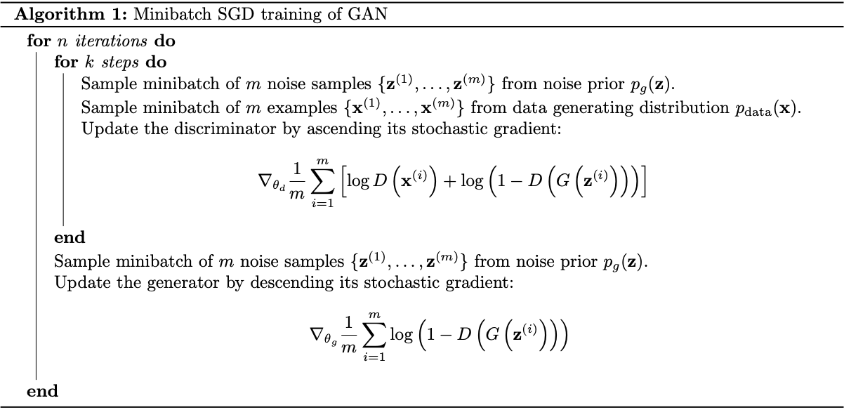
Training GAN

We will apply the minibatch SGD method for training GAN.

Wasserstein GAN (WGAN)

Wasserstein is a variation of GAN which use Wasserstein metric to measure the distance between probability distributions $p_r$ and $p_g$ instead of the Jensen-Shannon divergence.

Different Distances

Let $\mathcal{X}$ be a compact metric set, $\Sigma$ be the set of all the Borel subsets of $\mathcal{X}$ and let $\text{Prob}(\mathcal{X})$ denote the space of probability measures defined on $\mathcal{X}$. We can now define elementary distances and divergences between two probability distributions $P_r,P_g\in\text{Prob}(\mathcal{X})$

• Total Variation (TV) distance \begin{equation} \delta(P_r,P_g)=\sup_{A\in\Sigma}\big\vert P_r(A)-P_g(A)\big\vert \end{equation}
• Kullback-Leibler (KL) divergence \begin{equation} D_\text{KL}(P_r\Vert P_g)=\int_\mathcal{X}p_r(x)\log\frac{p_r(x)}{p_g(x)}d\mu(x), \end{equation} where both $P_r,P_g$ are assumed to be absolutely continuous, and therefore admit densities, w.r.t a measure $\mu$². The divergence is not symmetric and infinite when there are points such that $P_g(x)=0$ and $P_r(x)>0$.
• Jensen-Shannon (JS) divergence \begin{equation} D_\text{JS}(P_r\Vert P_g)=\frac{1}{2}D_\text{KL}(P_r\Vert P_m)+\frac{1}{2}D_\text{KL}(P_g\Vert P_m) \end{equation} where $P_m$ is the mixture distribution $P_m=\frac{P_r+P_g}{2}$. The divergence is symmetric.
• Earth Mover (EM) distance, or Wasserstein-1 \begin{equation} W(P_r,P_g)=\inf_{\gamma\in\Pi(P_r,P_g)}\mathbb{E}_{(x,y)\sim\gamma}\big[\Vert x-y\Vert_2\big]\label{eq:dd.1}, \end{equation} where $\Pi(P_r,P_g)$ is the set of all joint distribution $\gamma(x,y)$ whose marginal distributions are $P_r$ and $P_g$.

Example: Learning parallel lines

Consider probability distributions defined on $\mathbb{R}^2$:

• $P_0$ is the distribution of $(0,Y)$ where $Y\sim\text{Unif}(0,1)$.
• $P_\theta$ is the family of distribution of $(\theta,Y)$ with $Y\sim\text{Unif}(0,1)$.

Our goal is to learn to move from $\theta$ to $0$, i.e. as $\theta$ approaches $0$, the distance or divergence $d(P_0,P_\theta)$ tends to $0$. For each distance, or divergence we have

• TV distance. If $\theta=0$ then $P_0=P_\theta$, and thus \begin{equation} \delta(P_0,P_\theta)=\sup_{A\in\Sigma}\vert P_0(A)-P_\theta(A)\vert=0 \end{equation} If $\theta\neq 0$, let $\bar{A}=\{(0,y):y\in[0,1]\}$, we have \begin{equation} \delta(P_0,P_\theta)=\sup_{A\in\Sigma}\vert P_0(A)-P_\theta(A)\vert\geq\vert P_0(\bar{A})-P_\theta(\bar{A})\vert=1 \end{equation} Also, by definition we also have that $0\leq\delta(P_0,P_\theta)\leq 1$. Hence, for $\theta\neq 0,\delta(P_0,P_\theta)=1$. \begin{equation} \delta(P_0,P_\theta)=\begin{cases}0&\hspace{1cm}\text{if }\theta=0 \\ 1&\hspace{1cm}\text{if }\theta\neq 0\end{cases} \end{equation}
• KL divergence. By definition, we have that \begin{equation} D_\text{KL}(P_0\Vert P_\theta)=\begin{cases}0&\hspace{1cm}\text{if }P_0=P_\theta \\ +\infty&\hspace{1cm}\text{if }!x\in\mathbb{R}^2:P_0(x)>0,P_\theta(x)=0\end{cases} \end{equation} Therefore, we have that when $\theta\neq 0$, for any $a\in[0,1]$, \begin{equation} D_\text{KL}(P_0\Vert P_\theta)=+\infty, \end{equation} since $P_0(0,a)>0$ and $P_\theta(0,a)=0$, and \begin{equation} D_\text{KL}(P_\theta\Vert P_0)=+\infty, \end{equation} since $P_\theta(\theta,a)>0$ while $P_0(\theta,a)=0$. Therefore, it follows that \begin{equation} D_\text{KL}(P_0\Vert P_\theta)=D_\text{KL}(P_\theta\Vert P_0)=\begin{cases}0&\hspace{1cm}\text{if }\theta=0 \\ +\infty&\hspace{1cm}\text{if }\theta\neq 0\end{cases} \end{equation}
• JS divergence. It is easy to see that for $\theta=0$, we have $D_\text{JS}(P_0\Vert P_\theta)=0$. Let us consider the case that $\theta\neq 0$. Let $P_m$ denote the mixture $\frac{P_0+P_\theta}{2}$, we have \begin{equation} D_\text{JS}(P_0\Vert P_\theta)=\frac{1}{2}D_\text{KL}(P_0\Vert P_m)+\frac{1}{2}D_\text{KL}(P_\theta\Vert P_m) \end{equation} Consider the first KL divergence, we have that \begin{align} D_\text{KL}(P_0\Vert P_m)&=\int_{x}\int_{0}^{1}P_0(x,y)\log\frac{P_0(x,y)}{P_m(x,y)}\,dy\,dx \\ &\overset{\text{(i)}}{=}\int_{0}^{1}P_0(0,y)\log\frac{2P_0(0,y)}{P_0(0,y)+P_\theta(0,y)}\,dy\nonumber \\ &+\int_{0}^{1}\int_{x\neq 0}P_0(x,y)\log\frac{2P_0(x,y)}{P_0(x,y)+P_\theta(x,y)}\,dx\,dy \\ &\overset{\text{(ii)}}{=}\int_{0}^{1}P_0(0,y)\log 2\,dy+\int_{0}^{1}0\,dy \\ &=\log 2\int_{0}^{1}P_0(0,y)\,dy \\ &\overset{\text{(iii)}}{=}\log 2, \end{align} where
  • In this step, we use the Fubini's theorem to exchange the order of integration.
  • In this step, we use the fact that for any $y\in[0,1],P_0(0,y)>0$ while $P_\theta(0,y)=0$ and for any $x\neq 0,P_0(x,y)=0$.
  • In this step, the expression inside the integration integrates to $1$ since $P_0$ is a probability distribution.
  Similarly, we also have that \begin{equation} D_\text{KL}(P_\theta\Vert P_m)=\log 2 \end{equation} Therefore, it follows that \begin{equation} D_\text{JS}(P_0\Vert P_\theta)=\begin{cases}0&\hspace{1cm}\text{if }\theta=0 \\ \log 2&\hspace{1cm}\text{if }\theta\neq 0\end{cases} \end{equation}
• EM distance.

In other words,

• As $\theta_t\to 0$, the sequence $(P_{\theta_t})_{t\in\mathbb{N}}$ converges to $P_0$ under the EM distance, but does not converge under either the TV, KL, reverse KL or JS divergences.
• If we consider these distances and divergences as functions of $P_0$ and $P_\theta$, it is easily seen that EM is continuous, while none of the others is.

Remark: The example shows that

• There exist sequences of distributions that do not converge under either TV, KL, reverse KL or JS divergences but do converge under the EM distance.
• There are cases where EM is continuous everywhere, while all of the others are discontinuous.

Convergence and continuity of Wasserstein distance

Let $(X,d_X)$ and $(Y,d_Y)$ be two metric spaces. A function $f:X\mapsto Y$ is called Lipschitz continuous if there exists a constant $K\geq 0$ such that, for all $x_1,x_2\in X$, \begin{equation} d_Y(f(x_1),f(x_2))\leq K d_X(x_1,x_2) \end{equation} In this case, $K$ is known as a Lipschitz constant for $f$, while $f$ is referred to as K-Lipschitz. If $K=1$, $f$ is called a short map (or weak contraction). And if $0\leq K<1$ and $f$ maps a metric to itself, i.e. $X=Y,$ then $f$ is called a contraction.

The function $f$ is called locally Lipschitz continuous if $\forall x\in X$, there exists a neighborhood³ $U$ of $x$ such that $f$ restricted⁴ to $U$ is Lipschitz continuous.

Equivalently, if $X$ is a locally compact⁵ metric space, then $f$ is locally Lipschitz iff it is Lipschitz continuous on every compact subset of $X$.

Assumption 1
Let $g:\mathcal{Z}\times\mathbb{R}^d\mapsto\mathcal{X}$ be locally Lipschitz between finite dimensional vector spaces⁶ and denote $g_\theta(z)\doteq g(z,\theta)$. We say that $g$ satisfies Assumption 1 for a certain probability $p$ over $\mathcal{Z}$ if there are local Lipschitz constants $L(\theta,z)$ such that \begin{equation} \mathbb{E}_{z\sim p}\big[L(\theta,z)\big]\leq+\infty \end{equation}

Theorem 1
Let $P_r$ be a fixed distribution over $\mathcal{X}$ and $Z$ be a r.v over another space $\mathcal{Z}$. Let $g:\mathcal{Z}\times\mathbb{R}^d\mapsto\mathcal{X}$ with $g_\theta(z)\doteq g(\theta,z)$. And let $P_\theta$ denote the distribution of $g_\theta(Z)$. Then

• If $g$ is continuous in $\theta$, so is $W(P_r,P_\theta)$.
• If $g$ is locally Lipschitz and satisfies Assumption 1, then $W(P_r,P_\theta)$ is continuous everywhere, and differentiable almost everywhere.
• Statements (1) and (2) are false for the JS divergence $D_\text{JS}(P_r\Vert P_\theta)$, the KL divergence $D_\text{KL}(P_r\Vert P_\theta)$ and the reverse KL divergence $D_\text{KL}(P_\theta\Vert P_r)$.

Proof
TODO

We can apply this result to neural networks, as following.

Corollary 1
Let $g_\theta$ be any feedforward neural network parameterized by $\theta$, and let $p(z)$ be a prior over $z$ such that $\mathbb{E}_{z\sim p(z)}\big[\Vert z\Vert_2\big]\leq\infty$ (e.g. Gaussian, uniform, etc). Then Assumption 1 is satisfied and therefore $W(P_r,P_\theta)$ is continuous everywhere and differentiable almost everywhere.

Proof
TODO

Theorem 2
Let $P$ be a distribution on a compact space $\mathcal{X}$ and $(P_n)_{n\in\mathbb{N}}$ be a sequence of distribution on $\mathcal{X}$. Then, as $n\to\infty$,

• The following statements are equivalent
  • $\delta(P_n,P)\to 0$.
  • $D_\text{JS}(P_n\Vert P)\to 0$.
• The following statements are equivalent
  • $W(P_n,P)\to 0$.
  • $P_n\overset{\mathcal{D}}{\to}P$ where $\overset{\mathcal{D}}{\to}$ denotes convergence in distribution for r.v.s.
• $D_\text{KL}(P_n\Vert P)\to 0$ or $D_\text{KL}(P\Vert P_n)\to 0$ imply the statements in (1).
• The statements in (1) imply the statements in (2).

In other words, the theorem states that every distributions that converges under the TV, KL, reverse KL and JS divergences also converges under the Wasserstein distance.

Proof
TODO

Wasserstein GAN

Despite of having such nice properties, the infimum when computing EM distance \eqref{eq:dd.1} \begin{equation} W(P_r,P_g)=\inf_{\gamma\sim\Pi(P_r,P_g)}\mathbb{E}_{(x,y)\sim\gamma}\big[\Vert x-y\Vert_2\big] \end{equation} is however intractable. This suggests us to compute an approximation instead.

Theorem 3 (Kantorovich-Rubinstein duality)
\begin{equation} W(P_r,P_\theta)=\sup_{\Vert f\Vert_L\leq 1}\mathbb{E}_{x\sim P_r}[f(x)]-\mathbb{E}_{x\sim P_\theta}[f(x)] \end{equation}

Proof
Let $\mathcal{X}$ be a compact metric and let $\text{Prob}(\mathcal{X})$ denote the space of probability measures defined on $\mathcal{X}$. Let us consider two probability distribution $P_r,P_\theta\in\text{Prob}(\mathcal{X})$ with densities $p_r,p_\theta$ respectively. Let $\Pi(P_r,P_\theta)$ be the sets of all joint distribution $\gamma(x,y)$ whose marginals are respectively $P_r$ and $P_\theta$, i.e. \begin{align} p_r(x)&=\int_\mathcal{X}\gamma(x,y)\hspace{0.1cm}dy,\label{eq:wgan.1} \\ p_\theta(y)&=\int_\mathcal{X}\gamma(x,y)\hspace{0.1cm}dx\label{eq:wgan.2} \end{align} Their Wasserstein distance is given as \begin{equation} W(P_r,P_\theta)=\inf_{\gamma\in\Pi(P_r,P_\theta)}\mathbb{E}_{(x,y)\sim\gamma}\big[\Vert x-y\Vert_2\big], \end{equation} which is a convex optimization problem with constrains given in \eqref{eq:wgan.1} and \eqref{eq:wgan.2}. Let $f,g:\mathcal{X}\mapsto\mathbb{R}$ be Lagrange multipliers, the Lagrangian is then given as \begin{align} \hspace{-1cm}\mathcal{L}(\gamma,f,g)&=\mathbb{E}_{(x,y)\sim\gamma}\big[\Vert x-y\Vert_2\big]+\int_\mathcal{X}\left(p_r(x)-\int_\mathcal{X}\gamma(x,y)\hspace{0.1cm}dy\right)f(x)\hspace{0.1cm}dx \nonumber\\ &\hspace{4cm}+\int_\mathcal{X}\left(p_\theta(y)-\int_\mathcal{X}\gamma(x,y)\hspace{0.1cm}dx\right)g(y)\hspace{0.1cm}dy \\ &=\mathbb{E}_{x\sim P_r}\big[f(x)\big]+\mathbb{E}_{y\sim P_\theta}\big[g(y)\big]+\int_{\mathcal{X}\times\mathcal{X}}\gamma(x,y)\Big(\Vert x-y\Vert_2-f(x)-g(y)\Big)\hspace{0.1cm}dy\hspace{0.1cm}dx \end{align} Applying strong duality (?? TODO), we have \begin{equation} W(P_r,P_\theta)=\inf_\gamma\sup_{f,g}\mathcal{L}(\gamma,f,g)=\sup_{f,g}\inf_\gamma\mathcal{L}(\gamma,f,g) \end{equation}

TODO

If we replace $\Vert f\Vert_L\leq 1$ by $\Vert f\Vert_L\leq K$ (i.e. we instead consider the supremum over K-Lipschitz functions)

Preferences

[1] Ian J. Goodfellow, Jean Pouget-Abadie, Mehdi Mirza, Bing Xu, David Warde-Farley, Sherjil Ozair, Aaron Courville, Yoshua Bengio. Generative Adversarial Nets. NIPS, 2014.

[2] Martin Arjovsky, Soumith Chintala, Léon Bottou. Wasserstein GAN. arXiv preprint, arXiv:1701.07875, 2017.

[3] Alex Irpan. Read-through: Wasserstein GAN. Sorta Insightful.

[4] Elias M. Stein & Rami Shakarchi. Real Analysis: Measure Theory, Integration, and Hilbert Spaces. Princeton University Press, 2007.

Footnotes