The Exponential Family, Generalized Linear Models

Notes on Exponential Family & Generalized Linear Models.

The Exponential Family

The exponential family of distributions is defined as family of distributions of form \begin{align} p(x;\eta)&=h(x)\exp\Big[\eta^\text{T}T(x)-A(\eta)\Big],\label{eq:ef.1} \\ &= \frac{1}{Z(\eta)}h(x)\exp\Big[\eta^\text{T}T(x)\Big] \end{align} where

• $\eta$ is known as the natural parameter, or canonical parameter,
• $T(X)$ is referred to as a sufficient statistic,
• $A(\eta)$ is called the cumulant function, which can be view as the logarithm of a normalization factor (or partition function) $Z(\eta)$, i.e. $A(\eta)=\log Z(\eta)$, since integrating \eqref{eq:ef.1} w.r.t the measure $\nu$ gives us \begin{equation} A(\eta)=\log\int h(x)\exp\left(\eta^\text{T}T(x)\right)\nu(dx),\label{eq:ef.2} \end{equation} This also implies that $A(\eta)$ will be determined once we have specified $\nu,T(x)$ and $h(x)$.

The set of parameters $\eta$ for which the integral in \eqref{eq:ef.2} is finite is known as the natural parameter space \begin{equation} \mathcal{N}=\left\{\eta:\int h(x)\exp\left(\eta^\text{T}T(x)\right)\nu(dx)<\infty\right\} \end{equation} which explains why $\eta$ is also referred as natural parameter. If $\mathcal{N}$ is an non-empty open set, the exponential family is said to be a linear exponential family.

An exponential family is known as minimal if there are no linear constraints among the components of $\eta$ nor are there linear constraints among the components of $T(x)$. A linear exponential family in a minimal representation is referred as regular exponential family.

Examples

Each particular choice of $\nu$, $T$ and $h$ defines a family (or set) of distributions that is parameterized by $\eta$. As we vary $\eta$, we then get different distributions within this family.

Bernoulli distribution

The probability mass function (i.e., the density function w.r.t counting measure) of a Bernoulli random variable $X$, denoted as $X\sim\text{Bern}(\pi)$, is given by \begin{align} p(x;\pi)&=\pi^x(1-\pi)^{1-x} \\ &=\exp\big[x\log\pi+(1-x)\log(1-\pi)\big] \\ &=\exp\left[\log\left(\frac{\pi}{1-\pi}\right)x+\log(1-\pi)\right], \end{align} which can be written in the form of an exponential family distribution \eqref{eq:ef.1} with \begin{align} \eta&=\frac{\pi}{1-\pi} \\ T(x)&=x \\ A(\eta)&=-\log(1-\pi)=\log(1+e^{\eta}) \\ h(x)&=1 \end{align} Notice that the relationship between $\eta$ and $\pi$ is invertible since \begin{equation} \pi=\frac{1}{1+e^{-\eta}}, \end{equation} which is the sigmoid function.

Binomial distribution

The probability mass function of a Binomial random variable $X$, denoted as $X\sim\text{Bin}(N,\pi)$, is defined as \begin{align} p(x;N,\pi)&={N\choose x}\pi^{x}(1-\pi)^{1-x} \\ &={N\choose x}\exp\big[x\log\pi+(1-x)\log(1-\pi)\big] \\ &={N\choose x}\exp\left[\log\left(\frac{\pi}{1-\pi}\right)x+\log(1-\pi)\right], \end{align} which is in form of an exponential family distribution \eqref{eq:ef.1} with \begin{align} \eta&=\frac{\pi}{1-\pi} \\ T(x)&=x \\ A(\eta)&=-\log(1-\pi)=\log(1+e^{\eta}) \\ h(x)&={N\choose x} \end{align} Similar to the Bernoulli case, we also have the invertible relationship between $\eta$ and $\pi$ as \begin{equation} \pi=\frac{1}{1+e^{-\eta}} \end{equation}

Poisson distribution

The probability mass function of a Poisson random variable $X$, denoted as $X\sim\text{Pois}(\lambda)$, is given as \begin{align} p(x;\lambda)&=\frac{\lambda^x e^{-\lambda}}{x!} \\ &=\frac{1}{x!}\exp\left(x\log\lambda-\lambda\right), \end{align} which is also able to be written as an exponential family distribution \eqref{eq:ef.1} with \begin{align} \eta&=\log\lambda \\ T(x)&=x \\ A(\eta)&=\lambda=e^{\eta} \\ h(x)&=\frac{1}{x!} \end{align} Analogy to Bernoulli distribution, we also have that \begin{equation} \lambda=e^{\eta} \end{equation}

Gaussian distribution

The (univariate) Gaussian density of a random variable $X$, denoted as $X\sim\mathcal{N}(\mu,\sigma^2)$, is given by \begin{align} p(x;\mu,\sigma^2)&=\frac{1}{\sqrt{2\pi}\sigma}\exp\left[-\frac{(x-\mu)^2}{2\sigma^2}\right] \\ &=\frac{1}{\sqrt{2\pi}}\exp\left[\frac{\mu}{\sigma^2}x-\frac{1}{2\sigma^2}x^2-\frac{1}{2\sigma^2}\mu^2-\log\sigma\right], \end{align} which allows us to write it as an instance of the exponential family with \begin{align} \eta&=\left[\begin{matrix}\mu/\sigma^2 \\ -1/2\sigma^2\end{matrix}\right] \\ T(x)&=\left[\begin{matrix}x\\ x^2\end{matrix}\right] \\ A(\eta)&=\frac{\mu^2}{2\sigma^2}+\log\sigma=-\frac{\eta_1^2}{4\eta_2}-\frac{1}{2}\log(-2\eta_2) \\ h(x)&=\frac{1}{\sqrt{2\pi}} \end{align}

Multinomial distribution

Let $\mathbf{X}=(X_1,\ldots,X_K)$ be the collection of $K$ random variable in which $X_k$ denotes the number of times the $k$-th event occurs in a set of $N$ independent trials. And let $\mathbf{\pi}=(\pi_1,\ldots,\pi_K)$ with $\sum_{k=1}^{K}\pi_k=1$ correspondingly represents the probability of occurring of each event within each trials.

Then $\mathbf{X}$ is said to have Multinomial distribution, denoted as $\mathbf{X}\sim\text{Mult}_K(N,\boldsymbol{\pi})$, if its probability mass function is given as with $\sum_{k=1}^{K}x_k=1$ \begin{align} p(\mathbf{x};\boldsymbol{\pi},N,K)&=\frac{N!}{x_1!x_2!\ldots x_K!}\pi_1^{x_1}\pi_2^{x_2}\ldots\pi_n^{x_n} \\ &=\frac{N!}{x_1!x_2!\ldots x_K!}\exp\left(\sum_{k=1}^{K}x_k\log\pi_k\right)\label{eq:m.1} \end{align} It is noticeable that the above equation is not minimal, since there exists a linear constraint between the components of $T(\mathbf{x})$, which is \begin{equation} \sum_{k=1}^{K}x_k=1 \end{equation} In order to remove this constraint, we substitute $1-\sum_{k=1}^{K-1}x_k$ to $x_K$ , which lets \eqref{eq:m.1} be written by \begin{align} \hspace{-0.8cm}p(\mathbf{x};\boldsymbol{\pi},N,K)&=\frac{N!}{x_1!x_2!\ldots x_K!}\exp\left(\sum_{k=1}^{K}x_k\log\pi_k\right) \\ &=\frac{N!}{x_1!x_2!\ldots x_K!}\exp\left[\sum_{k=1}^{K-1}x_k\log\pi_k+\left(1-\sum_{k=1}^{K-1}x_k\right)\log\left(1-\sum_{k=1}^{K-1}\pi_k\right)\right] \\ &=\frac{N!}{x_1!x_2!\ldots x_K!}\exp\left[\sum_{i=1}^{K-1}\log\left(\frac{\pi_i}{1-\sum_{k=1}^{K-1}\pi_k}\right)x_i+\log\left(1-\sum_{k=1}^{K-1}\pi_k\right)\right]\label{eq:m.2} \end{align} With this representation, and also for convenience, for $i=1,\ldots,K$ we continue by letting \begin{equation} \eta_i=\log\left(\frac{\pi_i}{1-\sum_{k=1}^{K-1}\pi_k}\right)=\log\left(\frac{\pi_i}{\pi_K}\right)\label{eq:m.3} \end{equation} Take the exponential of both sides and summing over $K$, we have \begin{equation} \sum_{i=1}^{K}e^{\eta_i}=\frac{\sum_{i=1}^{K}\pi_i}{\pi_K}=\frac{1}{\pi_K}\label{eq:m.4} \end{equation} From this result, we have that the Multinomial distribution \eqref{eq:m.2} is therefore also a member of the exponential family with \begin{align} \eta&=\left[\begin{matrix}\log\left(\pi_1/\pi_K\right) \\ \vdots \\ \log\left(\pi_K/\pi_K\right)\end{matrix}\right] \\ T(\mathbf{x})&=\left[\begin{matrix}x_1,\ldots,x_K\end{matrix}\right]^\text{T} \\ A(\eta)&=-\log\left(1-\sum_{i=1}^{K-1}\pi_i\right)=-\log(\pi_K)=\log\left(\sum_{k=1}^{K}e^{\eta_k}\right) \\ h(\mathbf{x})&=\frac{N!}{x_1!x_2!\ldots x_K!} \end{align} Additionally, substituting the result \eqref{eq:m.4} into \eqref{eq:m.3} gives us for $i=1,\ldots,K$ \begin{equation} \eta_i=\log\left(\pi_i\sum_{k=1}^{K}e^{\eta_k}\right), \end{equation} or we can express $\boldsymbol{\pi}$ in terms of $\eta$ by \begin{equation} \pi_i=\frac{e^{\eta_i}}{\sum_{k=1}^{K}e^{\eta_k}}, \end{equation} which is the softmax function.

Multivariate Normal distribution

For the case of a multivariate Normal r.v $\mathbf{X}$, we have its PDF is given as \begin{align} p(\mathbf{x};\boldsymbol{\mu},\boldsymbol{\Sigma},K)&=\frac{1}{(2\pi)^{K/2}\vert\boldsymbol{\Sigma}\vert^{1/2}}\exp\left[-\frac{1}{2}(\mathbf{x}-\boldsymbol{\mu})^\text{T}\boldsymbol{\Sigma}^{-1}(\mathbf{x}-\boldsymbol{\mu})\right] \\ \end{align}

Convexity

Theorem 1: The natural space $\mathcal{N}$ is a convex set and the cumulant function $A(\eta)$ is a convex function. If the family is minimal, then $A(\eta)$ is strictly convex.

Proof
Let $\eta_1,\eta_2\in\mathcal{N}$, thus from \eqref{eq:ef.2}, we have that \begin{align} \exp\big(A(\eta_1)\big)&=A_1, \\ \exp\big(A(\eta_2)\big)&=A_2 \end{align} where $A_1,A_2$ are finite.

To prove that $\mathcal{N}$ is convex, we need to show that for any $\eta=\lambda\eta_1+(1-\lambda)\eta_2$ for $0\lt\lambda\lt 1$, we also have $\eta\in\mathcal{N}$. From \eqref{eq:ef.2}, and by Hölder’s inequality¹, we have \begin{align} \exp\big(A(\eta)\big)&=\int h(x)\exp\big(\eta^\text{T}T(x)\big)\nu(dx) \\ &=\int h(x)\exp\Big[\big(\lambda\eta_1+(1-\lambda)\eta_2\big)^\text{T}T(x)\Big]\nu(dx) \\ &=\int \Big[h(x)\exp\big(\eta_1^\text{T}T(x)\big)\Big]^{\lambda}\Big[h(x)\exp\big(\eta_2^\text{T}T(x)\big)\Big]^{1-\lambda}\nu(dx) \\ &\leq\Bigg[\int h(x)\exp\big(\eta_1^\text{T}T(x)\big)\nu(dx)\Bigg]^\lambda\Bigg[\int h(x)\exp\big(\eta_2^\text{T}T(x)\big)\nu(dx)\Bigg]^{1-\lambda} \\ &=\Big[\exp\big(A(\eta_1)\big)\Big]^\lambda\Big[\exp\big(A(\eta_2)\big)\Big]^{1-\lambda} \\ &=A_1^\lambda A_2^{1-\lambda},\label{eq:c.1} \end{align} which proves that $A(\eta)$ is finite, or $\eta\in\mathcal{N}$.

Moreover, taking logarithm of both sides of \eqref{eq:c.1} gives us \begin{equation} \lambda A(\eta_1)+(1-\lambda)A(\eta_2)\geq A(\eta)=A\big(\lambda\eta_1+(1-\lambda)\eta_2\big), \end{equation} which also claims the convexity of $A(\eta)$.

Additionally, by Hölder’s inequality, the equality in \eqref{eq:c.1} holds when \begin{equation} \Big[h(x)\exp\big(\eta_2^\text{T}T(x)\big)\Big]^{1-\lambda}=c\Big[h(x)\exp\big(\eta_1^\text{T}T(x)\big)\Big]^{\lambda(1/\lambda-1)} \end{equation} or \begin{equation} \exp\big(\eta_2^\text{T}T(x)\big)=c\exp\big(\eta_1^\text{T}T(x)\big), \end{equation} and therefore \begin{equation} (\eta_2-\eta_1)^\text{T}T(x)=\log c, \end{equation} which is not minimal since $\eta_1,\eta_2$ are taken arbitrarily.

Moments of sufficient statistic

In this section, we will see how the moments of the sufficient statistic $T(X)$ can be calculated from the cumulant function $A(\eta)$. In more specifically, the first moment (mean) and the second central moment (variance) of $T(X)$ are exactly the first and the second cumulants.

Let us first consider the first derivative of the cumulant function $A(\eta)$. By the dominated convergence theorem, we have \begin{align} \frac{\partial A(\eta)}{\partial\eta^\text{T}}&=\frac{\partial}{\partial\eta^\text{T}}\log\int\exp\big(\eta^\text{T}T(x)\big)h(x)\nu(dx) \\ &=\frac{\int T(x)\exp\big(\eta^\text{T}(x)\big)h(x)\nu(dx)}{\int\exp\big(\eta^\text{T}T(x)\big)h(x)\nu(dx)} \\ &=\int T(x)\exp\big(\eta^\text{T}T(x)-A(\eta)\big)h(x)\nu(dx)\label{eq:mv.1} \\ &=\int T(x)p(x;\eta)\nu(dx) \\ &=\mathbb{E}[T(X)],\label{eq:mv.2} \end{align} which is the mean of the sufficient statistic $T(X)$.

Moreover, taking the second derivative of cumulant function by continuing with the result \eqref{eq:mv.1}, we have \begin{align} \frac{\partial^2 A(\eta)}{\partial\eta\partial\eta^\text{T}}&=\frac{\partial}{\partial\eta^\text{T}}\int T(x)\exp\big(\eta^\text{T}T(x)-A(\eta)\big)h(x)\nu(dx) \\ &=\int T(x)\left(T(x)-\frac{\partial}{\partial\eta^\text{T}}A(\eta)\right)^\text{T}\exp\big(\eta^\text{T}T(x)-A(\eta)\big)h(x)\nu(dx) \\ &=\int T(x)\big(T(x)-E(T(X))\big)^\text{T}\exp\big(\eta^\text{T}T(x)-A(\eta)\big)h(x)\nu(dx) \\ &=\mathbb{E}\left[T(X)T(X)^\text{T}\right]-\mathbb{E}[T(X)]\mathbb{E}[T(X)]^\text{T} \\ &=\text{Var}[T(X)], \end{align} which is the variance (or the covariance matrix in the multivariate case) of the sufficient statistic $T(X)$, or the second central moment of of $T(X)$.

Accordingly, we have that the differentiating the cumulant function $A(\eta)$ to $n$-order gives us the $n$-th central moment of $T(X)$.

The expected value of $T(X)$, $\mu$, is also known as the mean parameter (or moment parameter). Additionally, since $\mu=\frac{\partial A(\eta)}{\partial\eta}$ and $A(\eta)$ is strictly convex (due to Theorem 1), then the relationship $\mu=\frac{\partial A(\eta)}{\partial\eta}$ is invertible, i.e. $\eta=\left(\frac{\partial A(\eta)}{\partial\eta}\right)^{-1}(\mu)$. More specifically, there exists a function $\psi$ which defines the one-to-one relationship between canonical parameter $\eta$ and moment parameter $\mu$, i.e. \begin{equation} \eta=\psi(\mu)\label{eq:mv.3} \end{equation} This implies that a distribution in the exponential family can be parameterized not only by the canonical parameter $\eta$, but also the mean parameter $\mu$.

Sufficiency

Let $X$ be a r.v and let $T(X)$ be a statistic. Suppose that the distribution of $X$ is parameterized by $\theta$, i.e. $p(x;\theta)$. Then $T(X)$ is said to be sufficient for $\theta$ if there is no information in $X$ regarding $\theta$ beyond that in $T(X)$. In other words, having observed $T(X)$, we can throw away $X$ for the purpose of inference w.r.t $\theta$. Specifically

• In Bayesian approach, $\theta$ is considered as a r.v. Thus, we say that $T(X)$ is sufficient for $\theta$ if \begin{equation} p\models(\theta\perp X\vert T(X)), \end{equation} which happens iff \begin{equation} p(\theta\vert T(x),x)=p(\theta\vert T(x)) \end{equation}
• In frequentist view, $\theta$ is considered as label rather than a r.v. Thus, $T(X)$ is sufficient for $\theta$ if the conditional distribution of $X$ given $T(X)$ is not a function of $\theta$, i.e. \begin{equation} p(x\vert T(x),\theta)=p(x\vert T(x)) \end{equation}
• For undirected models, the joint distribution can be described by a product of factors \begin{equation} p(x,T(x),\theta)=\psi_1(T(x),\theta)\psi_2(x,T(x)), \end{equation} where we have absorbed the partition function $Z$ in one of the potential functions. Moreover, since now $T(X)$ is a deterministic function of $X$, then $T(X)$ can be removed out from the LHS. Dividing both sides by $p(\theta)$ yields \begin{equation} p(x\vert\theta)=g(T(x),\theta)h(x,T(x))\label{eq:suf.1} \end{equation}

Sufficiency and the Exponential Family

An important feature of the exponential family is that its sufficient statistic can be obtained by simply observed, once the distribution is written in the form \eqref{eq:ef.1}. Recall that \begin{equation} p(x;\eta)=h(x)\exp\left[\eta^\text{T}T(x)-A(\eta)\right] \end{equation} From \eqref{eq:suf.1}, it follows immediately that $T(X)$ is a sufficient statistic for $\eta$.

MLE for Exponential Family

The reduction obtainable by using a sufficient statistic $T(X)$ is particularly notable in the case of i.i.d sampling.

Consider an i.i.d data set $\mathcal{D}=\{x_1,\ldots,x_N\}$, which is composed of $N$ independent r.v.s $X=(X_1,\ldots,X_N)$, characterized by the sample exponential family density. The likelihood function is then given by: \begin{align} L(\eta;\mathcal{D})=p(\mathbf{x}\vert\eta)&=\prod_{n=1}^{N}p(x_n\vert\eta) \\ &=\prod_{n=1}^{N}h(x_n)\exp\big[\eta^\text{T}T(x_n)-A(\eta)\big] \\ &=\left(\prod_{n=1}^{N}h(x_n)\right)\exp\left[\eta^\text{T}\left(\sum_{n=1}^{N}T(x_n)\right)-N A(\eta)\right]\label{eq:mle.1} \end{align} It is easily seen that $X$ is also an exponential distribution, with sufficient statistic $\sum_{n=1}^{N}T(x_n)$.

Taking the logarithm of both sides gives us the log likelihood as \begin{equation} \ell(\eta)=\log L(\eta)=\sum_{n=1}^{N}\log h(x_n)+\eta^\text{T}\left(\sum_{n=1}^{N}T(x_n)\right)-N A(\eta)\label{eq:mle.2} \end{equation} Consider the gradient of the log likelihood w.r.t $\eta$, we have \begin{align} \nabla_\eta\ell(\eta)&=\nabla_\eta\left[\sum_{n=1}^{N}\log h(x_n)+\eta^\text{T}\left(\sum_{n=1}^{N}T(x_n)\right)-N A(\eta)\right] \\ &=\sum_{n=1}^{N}T(x_n)-N\nabla_\eta A(\eta) \end{align} Setting the gradient to zero, we have the value of $\eta$ that maximizes the likelihood, or maximum likelihood estimation for $\eta$, denoted as $\hat{\eta}_\text{ML}$ satisfies \begin{equation} \nabla_{\eta}A(\hat{\eta}_\text{ML})=\frac{1}{N}\sum_{n=1}^{N}T(x_n) \end{equation} Finally, defining $\mu\doteq\mathbb{E}\big[T(X)\big]$. Then by \eqref{eq:mv.2}, we have that \begin{equation} \hat{\mu}_\text{ML}=\frac{1}{N}\sum_{n=1}^{N}T(x_n)\label{eq:mle.3} \end{equation} as the general formula for MLE of the mean parameter in the exponential family. And thus, by \eqref{eq:mv.3}, we obtain \begin{equation} \hat{\eta}_\text{ML}=\psi(\hat{\mu}_\text{ML}) \end{equation} It is worth noticing that the above formula involves the data only via the sufficient statistic $\sum_{n=1}^{N}T(x_n)$.

Example 1: From the result \eqref{eq:mle.3}, we have that

• For exponential family distribution with sufficient statistic $T(X)=X$, e.g. Bernoulli, Binomial, Poisson, the maximum likelihood estimate of the mean is exactly the sample mean, $\frac{1}{N}\sum_{n=1}^{N}x_n$.
• For univariate Normal distribution, which has $T(X)=\left[\begin{smallmatrix}X \\ X^2\end{smallmatrix}\right]$, the maximum likelihood estimate of the mean and variance are precisely the sample mean and sample variance.

MLE and the KL Divergence

Given a dataset $\mathcal{D}=\{x_1,\ldots,x_N\}$, the empirical distribution, denoted $\hat{p}(x)$, is a distribution which places probability mass $1/N$ at each data point $x_n$ in $\mathcal{D}$. In particular, \begin{equation} \hat{p}(x)\doteq\frac{1}{N}\sum_{n=1}^{N}\delta(x-x_n), \end{equation} where

• in the continuous case, $\delta(\cdot)$ is the Dirac delta function, which has zero-valued everywhere except $0$, and integrates to $1$.
• in the discrete case, $\delta(\cdot)$ is the Kronecker delta function, which takes value of $1$ at $0$, and zero elsewhere, and thus sums to $1$.

The following derivations is interchangeable between discrete and continuous circumstance by swapping between summation and integration. Thus, without loss of generality, let us consider the discrete case. Firstly, we have that \begin{align} \sum_x\hat{p}(x)\log p(x;\theta)&=\sum_x\frac{1}{N}\sum_{n=1}^{N}\delta(x-x_n)\log p(x;\theta) \\ &=\frac{1}{N}\sum_{n=1}^{N}\sum_x\delta(x-x_n)\log p(x;\theta) \\ &=\frac{1}{N}\sum_{n=1}^{N}\log p(x;\theta) \\ &=\frac{1}{N}\ell(\theta;\mathcal{D}) \end{align} where $\ell(\cdot)$ is the log-likelihood function.

On the other hand, consider the relative entropy, or KL divergence, between the empirical distribution and the model $p(x;\theta)$, we have that \begin{align} D_\text{KL}(\hat{p}(x)\Vert p(x;\theta))&=\sum_x\hat{p}(x)\log\left(\frac{\hat{p}(x)}{p(x;\theta)}\right) \\ &=\sum_x\hat{p}(x)\log\hat{p}(x)-\sum_x\hat{p}(x)\log p(x;\theta) \\ &=\mathbb{E}_{\hat{p}}\big[\log\hat{p}(x)\big]-\frac{1}{N}\ell(\theta;\mathcal{D}) \end{align} Since $\mathbb{E}_\hat{p}\big[\log\hat{p}(x)\big]$ does not depend on $\theta$, then the value of $\theta$ that minimizes the KL divergence to the empirical distribution is the one that maximizes the log-likelihood.

Conjugate priors

Given a probability distribution $p(x\vert\eta)$, its prior $p(\eta)$ is said to be conjugate to the likelihood function if the prior and the posterior has the same functional form. The prior distribution in this case is also referred as conjugate prior.

For any member of the exponential family, there exists a conjugate prior that can be written in form \begin{equation} p(\eta\vert\mathcal{X},\theta)=f(\mathcal{X},\theta)\exp(\eta^\text{T}\mathcal{X}-\theta A(\eta)),\label{eq:cp.1} \end{equation} where $\theta>0$ and $\mathcal{X}$ are hyperparameters.

By Bayes’ rule, and with the likelihood function as given in \eqref{eq:mle.1}, the posterior distribution can be computed as \begin{align} &\hspace{0.7cm}p(\eta\vert\mathbf{X},\mathcal{X},\theta) \\ &\propto p(\eta\vert\mathcal{X},\theta)p(\mathbf{X}\vert\eta) \\ &=f(\mathcal{X},\theta)\exp\big(\eta^\text{T}\mathcal{X}-\theta A(\eta)\big)\left(\prod_{n=1}^{N}h(x_n)\right)\exp\left[\eta^\text{T}\left(\sum_{n=1}^{N}T(x_n)\right)-N A(\eta)\right] \\ &\propto\exp\left[\eta^\text{T}\left(\mathcal{X}+\sum_{n=1}^{N}T(x_n)\right)-(\theta+N)A(\eta)\right], \end{align} which is in the same form as \eqref{eq:cp.1} and therefore claims the conjugacy.

Generalized Linear Models

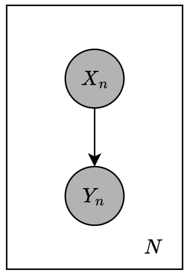
The generalized linear model (or GLIM) extends the idea of linear models in classification and regression to a more general settings using the definition of exponential family. Specifically, consider the plate model given below, which consists of two variables $X$ and $Y$ where both of them are assumed to be observed.

A GLIM makes threes assumptions about the conditional distribution $p(y\vert x)$

• The observed input $x$ is assumed to enter into the model via a linear combination $\xi=\theta^\text{T}x$.
• The conditional mean $\mu$ is represented as a function $f(\xi)$ of the linear combination $\xi$, where $f$ is referred as the response function, or link function.
• The observed output $y$ is assumed to be characterized by an exponential family distribution $p$ with conditional mean $\mu$.

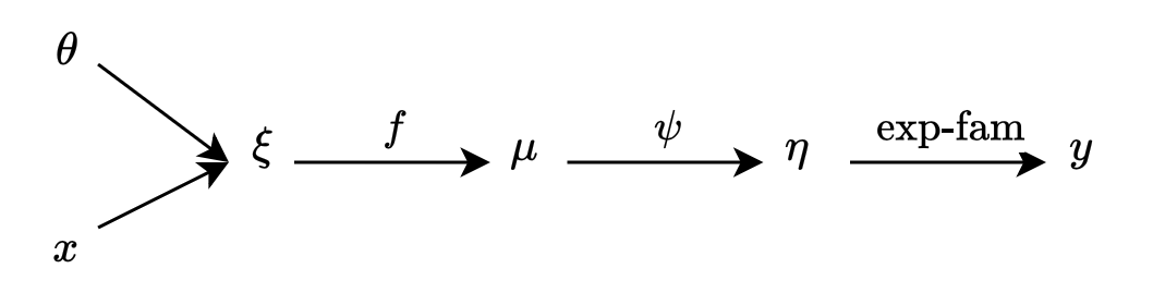
These assumption is summarized in the above figure. Notice that the diagram also provides us an invertible mapping from the mean parameter $\mu$ to the canonical parameter $\eta$, which we denote as $\eta=\psi(\mu)$. This allows us to use $\eta$ to represent the exponential family distribution for $Y$.

Formally, we assume that the output of GLIM has the form of \begin{equation} p(y;\eta,\phi)=h(y,\phi)\exp\left[\frac{\eta^\text{T}y-A(\eta)}{\phi}\right], \end{equation} which is slightly different from the traditional definition of exponential family density by including an explicit scale parameter $\phi$.

Additionally, since $\eta=\psi(\mu)$ and $\mu=f(\xi)=f(\theta^\text{T}x)$, then we directly have $\eta=\psi(f(\theta^\text{T}x))$. Thus, the conditional of $y$ given $x,\theta$ and $\phi$ is \begin{equation} p(y\vert x;\theta,\phi)=h(y,\phi)\exp\left[\frac{y^\text{T}\psi(f(\theta^\text{T}x))-A(\psi(\theta^\text{T}x))}{\phi}\right]\label{eq:glim.1} \end{equation} There are two principle choices in designing a GLIM: the choice of exponential family distribution and the choice of the response function $f(\cdot)$.

The former choice strongly depends on the pattern of $Y$. In particular, class labels are naturally represented by Bernoulli or Multinomial, counts by the Poisson, integrals by the exponential or Gamma distributions.

The latter choice has more degree of freedom with some mild constraints, e.g. in the case of Bernoulli and Multinomial, the conditional expectation must lie between $0$ and $1$, which suggests us to use a response function $f$ whose range is $(0,1)$; while we choose the response function $f$ with range $(0,\infty)$ for Gamma distribution, where the r.v is nonnegative. There is a particular choice called the canonical response function, which is $f(\cdot)=\psi^{-1}(\cdot)$. In this case, the conditional probability in \eqref{eq:glim.1} is simplified to \begin{equation} p(y\vert x;\theta,\phi)=h(y,\phi)\exp\left[\frac{y^\text{T}(\theta^\text{T}x)-A(\theta^\text{T}x)}{\phi}\right] \end{equation}

MLE for Generalized Linear Models with canonical response function

Consider an i.i.d dataset $\mathcal{D}=\{(x_1,y_1),\ldots,(x_N,y_N)\}$ where $y_n$ are scalars. The log-likelihood is then given as \begin{align} \ell(\theta;\mathcal{D})&=\log\prod_{n=1}^{N}p(y_n\vert x_n;\theta) \\ &=\sum_{n=1}^{N}\log\Big[h(y)\exp\big[\eta_n y_n-A(\eta_n)\big]\Big] \\ &=\sum_{n=1}^{N}\log h(y)+\sum_{n=1}^{N}\eta_n y_n-\sum_{n=1}^{N}A(\eta_n)\label{eq:mle-glm.1} \end{align} With canonical response function, which yields $\eta_n=\theta^\text{T}x_n$ for $n=1,\ldots,N$, the log-likelihood can be rewritten as \begin{align} p(y\vert x;\theta)&=\sum_{n=1}^{N}\log h(y)+\sum_{n=1}^{N}\theta^\text{T}y_n x_n-\sum_{n=1}^{N}A(\eta_n) \\ &=\sum_{n=1}^{N}\log h(y)+\theta^\text{T}\sum_{n=1}^{N}y_n x_n-\sum_{n=1}^{N}A(\eta_n) \end{align} Also, it is worth noticing that from \eqref{eq:mle.2}, we can see that $\sum_{n=1}^{N}x_n y_n$ is the sufficient statistic for $\theta$.

We continue by taking the derivative of the log-likelihood in \eqref{eq:mle-glm.1} w.r.t $\theta$ instead to get a more general form \begin{align} \nabla_\theta\ell(\theta;\mathcal{D})&=\sum_{n=1}^{N}\frac{d\ell(\theta;\mathcal{D})}{d\eta_n}\nabla_\theta\eta_n \\ &=\sum_{n=1}^{N}\left(y_n-\frac{d A(\eta_n)}{d\eta_n}\right)\frac{d\eta_n}{d\mu_n}\frac{d\mu_n}{d\xi_n}\nabla_\theta\xi_n \\ &=\sum_{n=1}^{N}(y_n-\mu_n)\frac{d\eta_n}{d\mu_n}\frac{d\mu_n}{d\xi_n}x_n\label{eq:mle-glm.2} \end{align} In using canonical response function, we have that $f=\psi^{-1}$, thus $\eta_n=\xi_n$, which implies that the derivative of the log-likelihood w.r.t can be simplified as \begin{equation} \nabla_\theta\ell(\theta;\mathcal{D})=\sum_{n=1}^{N}(y_n-\mu_n)x_n\label{eq:mle-glm.3} \end{equation}

Online updating

We then can use gradient ascent for estimating the parameter $\theta$, which has the update rule: \begin{equation} \theta^{(t+1)}=\theta^{(t)}+\rho(y_n-\mu_n^{(t)})x_n,\label{eq:mle-glm.4} \end{equation} where $\mu_n^{(t)}=f({\theta^{(t)}}^\text{T}x_n)$ and $\rho$ is the step size.

Notice that if our choice of $f$ is not the canonical response, \eqref{eq:mle-glm.4} is also a generic SGD algorithm for models throughout the GLIMs due to the fact that the derivatives of $f(\cdot)$ and $\psi(\cdot)$ in \eqref{eq:mle-glm.2}, i.e. $\frac{d\eta_n}{d\mu_n}$ and $\frac{d\mu_n}{d\xi_n}$, are absorbed into the step size $\rho$.

Batch updating

To using a batch algorithm, we start by vectorizing the gradient of the log-likelihood in \eqref{eq:mle-glm.3}, as \begin{align} \nabla_\theta\ell(\theta;\mathcal{D})&=\sum_{n=1}^{N}(y_n-\mu_n)x_n \\ &=X^\text{T}(y-\mu), \end{align} where $X$ is a matrix whose rows are $x_n^\text{T}$, and where $y,\mu$ are vectors whose components are $y_n$ and $\mu_n$ respectively, i.e. \begin{equation} \mathbf{X}=\left[\begin{matrix}-\hspace{0.1cm}x_1^\text{T}\hspace{0.1cm}- \\ \hspace{0.1cm}\vdots\hspace{0.1cm} \\ -\hspace{0.1cm}x_N^\text{T}\hspace{0.1cm}-\end{matrix}\right],\hspace{1cm}y=\left[\begin{matrix}y_1 \\ \vdots \\ y_N\end{matrix}\right],\hspace{1cm}\mu=\left[\begin{matrix}\mu_1 \\ \vdots \\ \mu_N\end{matrix}\right] \end{equation} Additionally, let us consider the Hessian matrix by taking the second derivative of the log-likelihood \begin{align} H_\ell&=\frac{\partial^2}{\partial\theta\partial\theta^\text{T}}\ell(\theta;\mathcal{D}) \\ &=\frac{\partial}{\partial\theta^\text{T}}\sum_{n=1}^{N}x_n(y_n-\mu_n) \\ &=-\sum_{n=1}^{N}x_n\frac{d\mu_n}{d\eta_n}\frac{\partial\eta_n}{\partial\theta^\text{T}} \\ &=\sum_{n=1}^{N}x_n\frac{d\mu_n}{d\eta_n}x_n^\text{T} \\ &=-X^\text{T}WX, \end{align} where $W$ is the diagonal weight matrix \begin{equation} W=\text{diag}\left(\frac{d\mu_1}{d\eta_1},\ldots,\frac{d\mu_N}{d\eta_N}\right), \end{equation} whose each diagonal entry can be computed via the second derivative of $A(\eta_n)$.

Using Newton’s method, we have the update rule \begin{align} \theta^{(t+1)}&=\theta^{(t)}-H_\ell^{-1}\nabla_\theta\ell \\ &=-H_\ell^{-1}(-H_\ell\theta^{(t)}+\nabla_\theta) \\ &=(X^\text{T}W^{(t)}X)^{-1}\big[X^\text{T}W^{(t)}X\theta^{(t)}+X^\text{T}(y-\mu^{(t)})\big] \\ &=(X^\text{T}W^{(t)}X)^{-1}X^\text{T}W^{(t)}z^{(t)},\label{eq:mle-glm.5} \end{align} where we have defined the adjusted response \begin{equation} z^{(t)}\doteq\eta+\big(W^{(t)}\big)^{-1}(y-\mu^{(t)}) \end{equation} This can be understood as solving the Iteratively Reweighted Least Squares (IRLS) problem \begin{equation} \theta^{(t)}=\underset{\theta}{\text{argmin}}(x-X\theta)^\text{T}\theta(z-X\theta) \end{equation}

References

[1] M. Jordan. The Exponential Family: Basics. 2009.

[2] Joseph K. Blitzstein & Jessica Hwang. Introduction to Probability.

[3] Weisstein, Eric W. Hölder’s Inequalities From MathWorld–A Wolfram Web Resource.

[4] Ian Goodfellow & Yoshua Bengio & Aaron Courville. Deep Learning. MIT Press, 2016.

Footnotes