Categorical Reparameterization with Gumbel-Softmax & Concrete Distribution

Notes on using Gumbel-Softmax & Concrete Distribution in Categorical sampling

Gumbel distribution

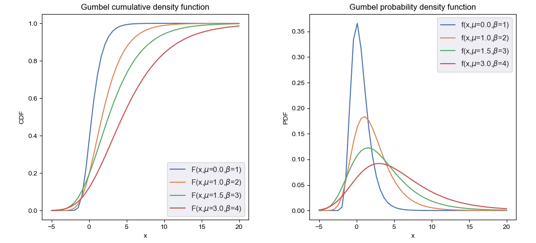
Gumbel distribution, denoted $\text{Gumbel}(\mu,\beta)$, is a continuous probability distribution whose cumulative density function (CDF) is given by \begin{equation} F(x)=\exp\left(-\exp\left(-\frac{x-\mu}{\beta}\right)\right), \end{equation} which implies that the probability density function (PDF) is given as \begin{equation} f(x)=F’(x)=\frac{1}{\beta}e^{-(e^{-z}+z)}, \end{equation} where \begin{equation} z=\frac{x-\mu}{\beta} \end{equation} The standard Gumbel distribution, denoted $\text{Gumbel}(0,1)$, is specified at location $\mu=0$ and unit scale $\beta=1$, whose density functions, i.e. CDF and PDF, are then explicitly given as \begin{align} F(x)&=e^{-e^{-x}} \\ f(x)&=e^{-(e^{-x}+x)}\label{eq:gd.1} \end{align} Below are some illustrations of Gumbel distribution.

Since the quantile function, i.e. inverse of the CDF, of Gumbel r.v $\text{Gumbel}(\mu,\beta)$ is referred as \begin{equation} Q(p)=\mu-\beta\log(-\log p), \end{equation} which implies that the standard Gumbel random variable $X\sim\text{Gumbel}(0,1)$ can be sampled using inverse transform sampling by first drawing $U\sim\text{Unif}(0, 1)$ and then computing \begin{equation} X=−\log(−\log U) \end{equation}

Optimizing Stochastic Computation Graph

Consider the following Stochastic Computation Graph

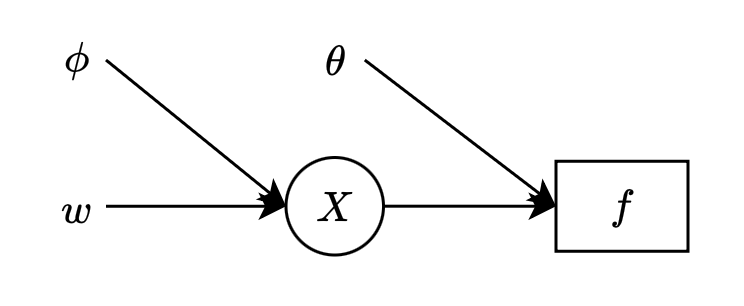
where

• $w,\phi,\theta$ denote input nodes.
• $X$ is a stochastic node, which is given by sampling according to $p_\phi(x\vert w)$.
• $f$ is a deterministic node, i.e. $f_\theta(x)$ is a deterministic function at $X$.

The graph corresponds to the objective function \begin{equation} L(\theta,\phi)=\mathbb{E}_{X\sim p_\phi(x)}\big[f_\theta(X)\big],\label{eq:oscg.1} \end{equation} where without loss of generality, we have considered $w$ as a constant.

Consider the backpropagation through the computation graph, we have that the gradient w.r.t $\theta$ of the cost function is given by \begin{equation} \nabla_\theta L(\theta,\phi)=\nabla_\theta\mathbb{E}_{X\sim p_\phi(x)}\big[f_\theta(X)\big]=\mathbb{E}_{X\sim p_\phi(x)}\big[\nabla_\theta f_\theta(X)\big],\label{eq:oscg.2} \end{equation} which, as an expectation, can be estimated using Monte Carlo method. In particular, let $X_1,\ldots,X_s$ be $s$ i.i.d samples drawn from $p_\phi(x)$, the gradient given in \eqref{eq:oscg.2} can be estimated with the unbiased \begin{equation} \nabla_\theta L(\theta,\phi)\approx\frac{1}{s}\sum_{i=1}^{s}\nabla_\theta f_\theta(X_i) \end{equation} On the other hands, taking the gradient w.r.t parameters $\phi$ gives us \begin{equation} \nabla_\phi L(\theta,\phi)=\nabla_\phi\int p_\phi(x)f_\theta(x)dx=\int f_\theta(x)\nabla_\phi p_\phi(x)dx,\label{eq:oscg.3} \end{equation} which can not be estimated directly using Monte Carlo sampling.

Score Function Estimators

Score function estimator utilizes the log-likelihood trick to rewrite the gradient in \eqref{eq:oscg.3} in an expectation form \begin{align} \nabla_\phi L(\theta,\phi)&=\int f_\theta(x)\nabla_\phi p_\phi(x)dx \\ &=\int f_\theta(x)p_\phi(x)\nabla_\phi\log p_\phi(x)dx \\ &=\mathbb{E}_{X\sim p_\phi(x)}\big[f_\theta(X)\nabla_\phi\log p_\phi(X)\big], \end{align} which analogously can be estimated by $s$ samples $X_1,\ldots,X_s\overset{\text{i.i.d}}{\sim} p_\phi(x)$ \begin{equation} \nabla_\phi L(\theta,\phi)\approx\frac{1}{s}\sum_{i=1}^{s}f_\theta(X_i)\nabla_\phi\log p_\phi(X_i) \end{equation}

Reparameterization Trick

In some circumstances, it could be helpful that instead of sampling from $p_\phi(x)$, we first sample $Z$ according to some fixed distribution $q(z)$ and then transform the sample to $x$ using some function $x=g_\phi(z)$.

For instance, by properties of the Normal distribution, a Gaussian sample $X\sim\mathcal{N}(\mu,\sigma^2)$ can always be obtained through a standard Normal $Z\sim\mathcal{N}(0,1)$ by computing $X=g_{\mu,\sigma}(Z)=\mu+\sigma Z$.

This reparameterization trick, $x=g_\phi(z)$, let us transfer the dependence on $\phi$ from $p$ into $f$ by writing \begin{equation} f_\theta(x)=f_\theta(g_\phi(z)), \end{equation} which enables the possibility of reducing the problem of estimating the gradient of w.r.t parameters of a distribution into a more trivial task of estimating the gradient w.r.t parameters of a deterministic function.

Applying this reparameterization trick allows us to rewrite the objective function given in \eqref{eq:oscg.1} as \begin{equation} L(\theta,\phi)=\mathbb{E}_{X\sim p_\phi(x)}\big[f_\theta(X)\big]=\mathbb{E}_{Z\sim q(z)}\big[f_\theta(g_\phi(Z))\big], \end{equation} which has the gradient w.r.t $\phi$ given by \begin{align} \nabla_\phi L(\theta,\phi)&=\nabla_\phi\mathbb{E}_{Z\sim q(z)}\big[f_\theta(g_\phi(Z))\big] \\ &=\mathbb{E}_{Z\sim q(z)}\big[\nabla_\phi f_\theta(g_\phi(Z))\big] \\ &=\mathbb{E}_{Z\sim q(z)}\big[f_\theta’(g_\phi(Z))\nabla_\phi g_\phi(Z)\big] \end{align}

Gumbel-Max Trick

Using the idea of reparameterization trick, Gumbel-Max trick refers to an approach that allows us to sample from a categorical distribution¹ through sampling according to Gumbel distribution.

First let $D$ be a categorical variable with class probabilities $\alpha_1,\alpha_2,\ldots,\alpha_k$ for $\sum_{i=1}^{k}\alpha_i=1$ and without loss of generality we can assume that zero category probability excluded, i.e. $\alpha_i>0$. Thus, we can express each sample drawn from the distribution as a $k$-dimensional one-hot vector lying in the corner (or vertex) of a $(k-1)$-dimensional probability simplex $\Delta^{k-1}$². In particular, each categorical sample is in form of \begin{equation} D=\left[\begin{matrix}D_1 \\ \vdots \\ D_k\end{matrix}\right], \end{equation} where $\sum_{i=1}^{k}D_i=1$; for $i=1,\ldots,k$ we have $D_i\in\{0,1\}$ and $P(D_i=1)=\alpha_i$.

Usually, we rewrite each class probability as a softmax function \begin{equation} \alpha_i=\frac{\exp(\pi_i)}{\sum_{j=1}^{k}\exp(\pi_j)} \end{equation} where $\pi_i\in(-\infty,0)$.

Gumbel-max trick provides us another way to get samples following this discrete distribution through samples drawn from Gumbel distribution. The trick is described as follow.

Consider $k$ unit-scaled Gumbel random variables $G_1,\ldots,G_k$ where $G_i\sim\text{Gumbel}(\pi_i,1)$. Thus, the density functions corresponds to $\text{Gumbel}(\pi_i,1)$ are given by \begin{equation} P(G_i\leq x)=F_{G_i}(x)=\exp(-\exp(-x+\pi_i)), \end{equation} and also its PDF \begin{equation} f_{G_i}(x)=\exp(-\exp(-x+\pi_i)-x+\pi_i) \end{equation} We have that the probability that $G_m$ taking the maximal value across $k$ samples can be computed as \begin{align} P\left(G_m=\max_{i=1,\ldots,k}G_i\Bigg\vert G_m=x\right)&=P\big(G_1\leq G_m,\ldots, G_k\leq G_m\big\vert G_m=x\big) \\ &=\prod_{i=1,i\neq m}^{k}P(G_i\leq G_m\vert G_m=x) \\ &=\prod_{i=1,i\neq m}^{k}F_{G_i}(x) \\ &=\prod_{i=1,i\neq m}^{k}\exp(-\exp(-x+\pi_i)) \end{align} Therefore, integrating over sample space of $G_m$, the probability that an arbitrary index $m$ corresponds to the largest sample $G_m$, i.e. $m=\text{argmax}_i G_i$ is computed by \begin{align} &P\left(m=\underset{i=1,\ldots,k}{\text{argmax}}G_i\right)\nonumber \\ &=\int f_m(x)\left(G_m=\max_{i=1,\ldots,k}G_i\Bigg\vert G_m=x\right)dx \\ &=\int\exp(-\exp(-x+\pi_m)-x+\pi_m)\prod_{i=1,i\neq m}^{k}\exp(-\exp(-x+\pi_i))dx \\ &=\int\exp(-x+\pi_m)\prod_{i=1}^{k}\exp(-\exp(-x+\pi_i))dx \\ &=\exp(\pi_m)\int\exp(-x)+\exp\Bigg(-\exp(-x)\sum_{i=1}^{k}\exp(\pi_i)\Bigg)dx \\ &=\frac{\exp(\pi_m)}{\sum_{i=1}^{k}\exp(\pi_i)}\int\exp(-\exp(-x)-x)dx\label{eq:gmt.1} \\ &=\frac{\exp(\pi_m)}{\sum_{i=1}^{k}\exp(\pi_i)}, \end{align} where the last step is due to that the integrand in \eqref{eq:gmt.1} is the PDF of a standard Gumbel distribution, as defined in \eqref{eq:gd.1}, which therefore integrates to $1$. Hence, we have that \begin{equation} P\left(m=\underset{i=1,\ldots,k}{\text{argmax}}G_i\right)=\pi_m \end{equation} Since a $\text{Gumbel}(\mu,\beta)$ can always be obtained from a standard $\text{Gumbel}(0,1)$ by scaling it with $\beta$ then translationing with $\mu$, then $G_i\sim\text{Gumbel}(\pi_i,1)$ can be computed as \begin{equation} G_i=g+\pi_i, \end{equation} where $g\sim\text{Gumbel}(0,1)$, which as mentioned above, can be obtained with \begin{equation} g=-\log(-\log u), \end{equation} where $u$ is drawn from an Uniform distribution, $u\sim\text{Unif}(0,1)$.

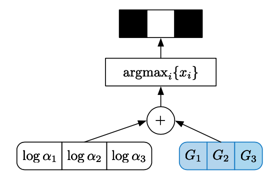
To summarize this, the Gumbel-max trick proceeds as: let \begin{equation} U_1,\ldots,U_k\overset{\text{i.i.d}}{\sim}\text{Unif}(0,1),\label{eq:gmt.2} \end{equation} and let \begin{equation} m=\underset{i=1,\ldots,k}{\text{argmax}}\log\alpha_i-\log(-\log U_i),\label{eq:gmt.3} \end{equation} where $\alpha=(\alpha_1,\alpha_2\ldots,\alpha_k)$ with $\alpha_i\in(0,\infty)$ is an unnormalized parameterization of a discrete distribution $D\sim\text{Discrete}(\alpha)$. Then each sample $D$ can be expressed as a one-hot vector \begin{equation} D=\left[\begin{matrix}D_1 \\ \vdots \\ D_k\end{matrix}\right], \end{equation} where $D_m=1$ and $D_i=0$ for $i=1,\ldots,k$ and $i\neq m$. Then \begin{equation} P(D_m=1)=\frac{\alpha_m}{\sum_{i=1}^{k}\alpha_i} \end{equation} The below figure illustrates the reparameterization sampling process.

Gumbel-Softmax & Concrete Distribution

Since $\text{argmax}$ function is non-differentiable (as illustrated by a discrete node in Figure 2), thus in order to apply the reparameterization in SCG, we use a continuous approximation of the function, which is the $\text{softmax}$ function, as visualized in Figure 3.

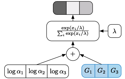
Rather than unit vectors (lying at the corners of $\Delta^{k-1}$), the resulting samples now are described in stochastic form (staying inside the probability simplex $\Delta^{k-1}$ instead). They follow to a distribution called Concrete, or Gumbel-Softmax. In particular, as illustrated above, to sample a Concrete random variable $X\in\Delta^{k-1}$ at temperature $\lambda\in(0,\infty)$ with parameter vector $\alpha=(a_1,\ldots,a_k)$ where $a_i\in(0,\infty)$, we first sample $G_i\overset{\text{i.i.d}}{\sim}\text{Gumbel}(0,1)$ and set \begin{equation} X_i=\frac{\exp((\log\alpha_i+G_i)/\lambda)}{\sum_{j=1}^{k}\exp((\log\alpha_j+G_j)/\lambda)}\label{eq:gsc.1} \end{equation} The $\text{softmax}$ computation of \eqref{eq:gsc.1} smoothly approaches the discrete $\text{argmax}$ computation as $\lambda\to 0$ while preserving the relative order of the Gumbels $\log\alpha_i+G_i$. At higher temperature, the Concrete samples are no longer one-hot, and as $\lambda\to\infty$, they become uniform.

The probability density function of a Concrete random variable $X\sim\text{Concrete}(\alpha,\lambda)$ with location vector $\alpha\in(0,\infty)^k$ and temperature $\lambda\in(0,\infty)$ is given as \begin{equation} f_X(x)=\Gamma(k)\lambda^{k-1}\prod_{i=1}^{k}\frac{\alpha_i x_i^{-\lambda-1}}{\sum_{j=1}^{k}\alpha_j x_j^{-\lambda}} \end{equation}

Proposition 1 (Properties of Concrete r.v.s) Let $X\sim\text{Concrete}(\alpha,\lambda)$ with location $\alpha\in(0,\infty)^k$ and temperature $\lambda\in(0,\infty)$. Then

• Reparameterization. If $G_i\overset{\text{i.i.d}}{\sim}\text{Gumbel}(0,1)$, then \begin{equation} X_i\overset{\text{d}}{=}\frac{\exp((\log\alpha_i+G_i)/\lambda)}{\sum_{j=1}^{k}\exp((\log\alpha_j+G_j)/\lambda)}, \end{equation} where $A\overset{\text{d}}{=}B$ denotes that random variables $A$ and $B$ follow the same distribution.
• Rounding. $P(X_i>X_m,i\neq m)=\frac{\alpha_i}{\sum_{j=1}^{k}\alpha_j}$
• Zero temperature. $P\left(\lim_{\lambda\to 0}X_i=1\right)=\frac{\alpha_i}{\sum_{j=1}^{k}\alpha_j}$
• Convex eventually. If $\lambda\leq(k-1)^{-1}$, then $f_X(x)$ is log-convex in $x$.

Proof

• Let $Y_i=\log\alpha_i+G_i$ for $i=1,\ldots,k$, then $Y_i$ are unit-scaled Gumbel r.v.s with locations $\log\alpha_i$, which have the PDFs given as \begin{align} f_{Y_i}(y_i)&=\exp(-\exp(-y_i+\log\alpha_i)-y_i+\log\alpha_i) \\ &=\alpha_i\exp(-y_i)\exp(-\alpha_i\exp(-y_i))\label{eq:gsc.2} \end{align} Also, let \begin{equation} Z_i=\frac{\exp((\log\alpha_i+G_i)/\lambda)}{\sum_{j=1}^{k}\exp((\log\alpha_j+G_j)/\lambda)}=\frac{\exp(Y_i/\lambda)}{\sum_{j=1}^{k}\exp(Y_j/\lambda)}, \end{equation} which implies that the r.v.s $Z_1,\ldots,Z_k$ relate to each other with the dependence \begin{equation} \sum_{i=1}^{k}Z_i=1 \end{equation} We continue by considering the invertible transformation \begin{equation} T(y_1,\ldots,y_k)=(z_1,\ldots,z_{k-1},c), \end{equation} where \begin{align} z_i&=\frac{1}{c}\exp\left(\frac{y_i}{\lambda}\right) \\ c&=\sum_{j=1}^{k}\exp\left(\frac{y_j}{\lambda}\right) \end{align} Hence, its inverse is given by \begin{align} \hspace{-1cm}T^{-1}(z_1,\ldots,z_{k-1},c)&=(y_1,\ldots,y_k) \\ &=(\lambda\log(z_1 c),\ldots,\lambda\log(z_{k-1}c),\lambda\log(z_k c)) \\ &=(\lambda(\log z_1+\log c),\ldots,\lambda(\log z_{k-1}+\log c),\lambda(\log z_k+\log c)), \end{align} where $z_k=1-\sum_{j=1}^{k-1}z_j$. Therefore, by change of variables \begin{align} f_{Z,C}(z_1,\ldots,z_k,c)&=f_{Z,C}(z_1,\ldots,z_{k-1},c) \\ &=f_Y(y_1,\ldots,y_k)\left\vert\text{det}\left(\frac{\partial Y}{\partial Z}\right)\right\vert\label{eq:gsc.3} \end{align} Let us consider the determinant of Jacobian matrix $\frac{\partial Y}{\partial Z}$, which can be computed by \begin{align} \hspace{-0.5cm}\text{det}\left(\frac{\partial Y}{\partial Z}\right)&=\text{det}\left[\begin{matrix}\lambda z_1^{-1}&0&0&0&\ldots&0&\lambda c^{-1} \\ 0&\lambda z_2^{-1}&0&0&\ldots&0&\lambda c^{-1} \\ 0&0&\lambda z_3^{-1}&0&\ldots&0&\lambda c^{-1} \\ \vdots&\vdots&\vdots&\vdots&\ddots&\vdots&\vdots \\ -\lambda z_k^{-1}&-\lambda z_k^{-1}&-\lambda z_k^{-1}&-\lambda z_k^{-1}&\ldots&-\lambda z_k^{-1}&\lambda c^{-1}\end{matrix}\right] \\ &=\text{det}\left[\begin{matrix}\lambda z_1^{-1}&0&0&0&\ldots&0&\lambda c^{-1} \\ 0&\lambda z_2^{-1}&0&0&\ldots&0&\lambda c^{-1} \\ 0&0&\lambda z_3^{-1}&0&\ldots&0&\lambda c^{-1} \\ \vdots&\vdots&\vdots&\vdots&\ddots&\vdots&\vdots \\ 0&0&0&0&\ldots&0&\lambda(z_k c)^{-1}\end{matrix}\right] \\ &=\frac{\lambda^k}{c\prod_{j=1}^{k}z_j} \end{align} Using the definition of PDFs of $Y_i$ given in \eqref{eq:gsc.2}, we can continue to derive \eqref{eq:gsc.3} as \begin{align} &f_{Z,C}(z_1,\ldots,z_k,c)\nonumber \\ &=f_Y(y_1,\ldots,y_k)\left\vert\text{det}\left(\frac{\partial Y}{\partial Z}\right)\right\vert \\ &=\left(\prod_{i=1}^{k}f_{Y_i}(y_i)\right)\frac{\lambda^k}{c\prod_{j=1}^{k}z_j} \\ &=\left(\prod_{i=1}^{k}f_{Y_i}\big(\lambda(\log z_i+\log c)\big)\right)\frac{\lambda^k}{c\prod_{j=1}^{k}z_j} \\ &=\frac{\lambda^k\prod_{i=1}^{k}\alpha_i\exp(-\lambda(\log z_i+\log c))\exp(-\alpha_i\exp(-\lambda(\log z_i+\log c)))}{c\prod_{j=1}^{k}z_j} \\ &=\frac{\lambda^k\prod_{i=1}^{k}\alpha_i}{c\prod_{j=1}^{k}z_j^{\lambda+1}}\exp(-k\lambda\log c)\exp\left(-\sum_{i=1}^{k}\alpha_i\exp(-\lambda\log z_i-\lambda\log c)\right) \\ &=\frac{\lambda^k\prod_{i=1}^{k}\alpha_i}{c\prod_{j=1}^{k}z_j^{\lambda+1}}\exp(-k\lambda\log c)\exp\left(-\exp(-\lambda\log c)\sum_{i=1}^{k}\alpha_i z_i^{-\lambda}\right) \end{align} Integrating the joint density $f_{Z,C}$ over $c$ and letting $\gamma=\log\sum_{i=1}^{k}\alpha_i z_i^{-\lambda}$ gives us the marginal distribution \begin{align} &f_Z(z_1,\ldots,z_k)\nonumber \\ &=\int_{0}^{\infty}\frac{\lambda^k\prod_{i=1}^{k}\alpha_i}{c\prod_{j=1}^{k}z_j^{\lambda+1}}\exp(-k\lambda\log c)\exp(-\exp(-\lambda\log c+\gamma))dc \\ &=\int_{0}^{\infty}\frac{\lambda^k\prod_{i=1}^{k}\alpha_i}{c\prod_{j=1}^{k}z_j^{\lambda+1}\exp(\gamma)}\exp(-k\lambda\log c+k\gamma)\exp(-\exp(-\lambda\log c+\gamma))dc \end{align} Let $u=\lambda\log c-\gamma$, so \begin{equation} du=d(\lambda\log c-\gamma))=\frac{\lambda}{c}dc, \end{equation} the above integration thus can be rewritten as \begin{equation} f_Z(z_1,\ldots,z_k)=\frac{\lambda^{k-1}\prod_{i=1}^{k}\alpha_i}{\prod_{j=1}^{k}z_j^{\lambda+1}\exp(\gamma)}\int_{-\infty}^{\infty}\exp(-ku)\exp(-\exp(-u))du \end{equation} Let $v=\exp(-u)$, then \begin{equation} dv=d(\exp(-u))=-\exp(-u)du, \end{equation} which implies that \begin{align} f_Z(z_1,\ldots,z_k)&=\frac{\lambda^{k-1}\prod_{i=1}^{k}\alpha_i}{\prod_{j=1}^{k}z_j^{\lambda+1}\exp(\gamma)}\int_{0}^{\infty}v^{k-1}\exp(-v)dv \\ &=\frac{\lambda^{k-1}\prod_{i=1}^{k}\alpha_i}{\prod_{j=1}^{k}z_j^{\lambda+1}\exp(\gamma)}\Gamma(k) \\ &=\Gamma(k)\lambda^{k-1}\prod_{i=1}^{k}\frac{\alpha_i z_i^{-\lambda-1}}{\sum_{j=1}^{k}\alpha_j z_j^{-\gamma}}, \end{align} which claims that $Z\overset{\text{d}}{=}X$.
• This follows directly from (i) and the Gumbel-Max trick
• This follows directly from (i) and the Gumbel-Max trick
• Let $\lambda\leq(k-1)^{-1}$. The density of $X$ can be rewritten as \begin{align} f_X(x)&=\Gamma(k)\lambda^{k-1}\prod_{i=1}^{k}\frac{\alpha_i x_i^{-\lambda-1}}{\sum_{j=1}^{k}\alpha_j x_j^{-\gamma}} \\ &=\Gamma(k)\lambda^{k-1}\prod_{i=1}^{k}\frac{\alpha_i x_i^{\lambda(k-1)-1}}{\sum_{j=1}^{k}\alpha_j\prod_{l\neq j}x_l^\lambda} \end{align} Thus, the log density of $X$ is given as \begin{align} \log f_X(x)&=\log\left(\Gamma(k)\lambda^{k-1}\prod_{i=1}^{k}\frac{\alpha_i x_i^{\lambda(k-1)-1}}{\sum_{j=1}^{k}\alpha_j\prod_{l\neq j}x_l^\lambda}\right) \\ &=\log(\Gamma(k)\lambda^{k-1})+\sum_{i=1}^{k}(\lambda(k-1)-1)\log x_i-k\log\left(\sum_{j=1}^{k}\alpha_j\prod_{l\neq j}x_l^\lambda\right), \end{align} which can be easily observed to be convex with $\lambda\leq(k-1)^{-1}$ due to $-\log$ function is convex and non-increasing and $\prod_{l\neq j}x_l^\lambda$ is concave, while the first term $\log(\Gamma(k)\lambda^{k-1})$ is a constant.

References

[1] Eric Jang, Shixiang Gu, Ben Poole. Categorical Reparameterization with Gumbel-Softmax. ICLR 2017.

[2] Chris J. Maddison, Andriy Mnih, Yee Whye Teh. The Concrete Distribution: A Continuous Relaxation of Discrete Random Variables. ICLR 2017.

[3] John Schulman, Theophane Weber, Nicolas Heess, Pieter Abbeel. Gradient Estimation Using Stochastic Computation Graphs. NIPS, 2015.

[4] Wikipedia. Gumbel distribution.

[5] Chris J. Maddison, Daniel Tarlow, Tom Minka. A$^*$ Sampling. NIPS, 2014.

Footnotes