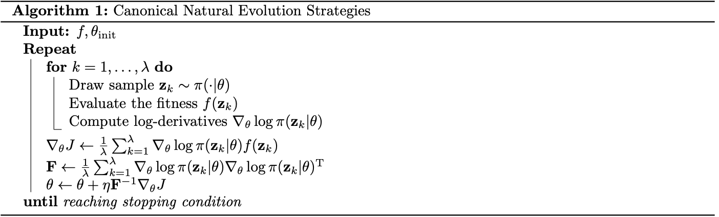
Natural Evolution Strategies, or NES, are referred to a family of evolution strategies that throughout its generations update a search distribution repeatedly using an estimated gradient of its distribution parameters.
Search gradients
Usually when working on Evolution Strategy methods, we select some candidate solutions, which generate better fitness values than the other ones, to be parents of the next generation. This means, majority of solution samples have been wasted since they may contain some useful information.
To utilize the use all fitness samples, the NES uses search gradients in updating the parameters for the search distribution.
Let $\mathbf{z}\in\mathbb{R}^n$ denote the solution sampled from the distribution $\pi(\mathbf{z},\theta)$ and let $f:\mathbb{R}^n\to\mathbb{R}$ be the fitness (or objective) function. The expected fitness value is then given by \begin{equation} J(\theta)=\mathbb{E}_\theta[f(\mathbf{z})]=\int f(\mathbf{z})\pi(\mathbf{z}\vert\theta)\hspace{0.1cm}d\mathbf{z}\label{eq:sg.1} \end{equation} Taking the gradient of the above function w.r.t $\theta$ using the log-likelihood trick as in REINFORCE gives us \begin{align} \nabla_\theta J(\theta)&=\nabla_\theta\int f(\mathbf{z})\pi(\mathbf{z}\vert\theta)\hspace{0.1cm}d\mathbf{z} \\ &=\int f(\mathbf{z})\nabla_\theta\pi(\mathbf{z}\vert\theta)\hspace{0.1cm}d\mathbf{z} \\ &=\int f(\mathbf{z})\nabla_\theta\pi(\mathbf{z}\vert\theta)\frac{\pi(\mathbf{z}\vert\theta)}{\pi(\mathbf{z}\vert\theta)}\hspace{0.1cm}d\mathbf{z} \\ &=\int\left[f(\mathbf{z})\nabla_\theta\log\pi(\mathbf{z}\vert\theta)\right]\pi(\mathbf{z}\vert\theta)\hspace{0.1cm}d\mathbf{z} \\ &=\mathbb{E}_\theta\left[f(\mathbf{z})\nabla_\theta\log\pi(\mathbf{z}\vert\theta)\right] \end{align} Using Monte Carlo method, given samples $\mathbf{z}_1,\ldots,\mathbf{z}_\lambda$ from the population of size $\lambda$, the search gradient is then can be approximated by \begin{equation} \nabla_\theta J(\theta)\approx\frac{1}{\lambda}\sum_{k=1}^{\lambda}f(\mathbf{z}_k)\nabla_\theta\log\pi(\mathbf{z}_k\vert\theta)\label{eq:sg.2} \end{equation} Given this gradient w.r.t $\theta$, we then can use a gradient-based method to repeatedly update the parameter $\theta$ in order to give us a more desired search distribution. In particular, we can use such as SGD method \begin{equation} \theta\leftarrow\theta+\alpha\nabla_\theta J(\theta),\label{eq:sg.3} \end{equation} where $\alpha$ is the learning rate.
Search gradients for MVN
Consider the case that our search distribution $\pi(\mathbf{z}\vert\theta)$ is in form of a Multivariate Normal distribution, $\mathbf{z}\sim\mathcal{N}(\boldsymbol{\mu},\boldsymbol{\Sigma})$, where $\boldsymbol{\mu}\in\mathbb{R}^n$ and $\boldsymbol{\Sigma}\in\mathbb{R}^{n\times n}$.
In this case $\theta=(\boldsymbol{\mu},\boldsymbol{\Sigma})$ denotes a tuple of parameters for the search distribution, which is given by \begin{equation} \pi(\mathbf{z}\vert\theta)=\frac{1}{(2\pi)^{n/1}\left\vert\boldsymbol{\Sigma}\right\vert^{1/2}}\exp\left[-\frac{1}{2}\left(\mathbf{z}-\boldsymbol{\mu}\right)^\text{T}\boldsymbol{\Sigma}^{-1}\left(\mathbf{z}-\boldsymbol{\mu}\right)\right] \end{equation} Taking natural logarithm of both sides then gives us \begin{align} \log\pi(\mathbf{z}\vert\theta)&=\log\left(\frac{1}{(2\pi)^{n/1}\left\vert\boldsymbol{\Sigma}\right\vert^{1/2}}\exp\left[-\frac{1}{2}\left(\mathbf{z}-\boldsymbol{\mu}\right)^\text{T}\boldsymbol{\Sigma}^{-1}\left(\mathbf{z}-\boldsymbol{\mu}\right)\right]\right) \\ &=-\frac{n}{2}\log(2\pi)-\frac{1}{2}\log\vert\boldsymbol{\Sigma}\vert-\frac{1}{2}\left(\mathbf{z}-\boldsymbol{\mu}\right)^\text{T}\boldsymbol{\Sigma}^{-1}\left(\mathbf{z}-\boldsymbol{\mu}\right) \end{align} We continue by differentiating the above log-likelihood w.r.t $\boldsymbol{\mu}$ and $\boldsymbol{\Sigma}$. Starting with $\boldsymbol{\mu}$, the gradient is given by \begin{align} \nabla_\boldsymbol{\mu}\log\pi(\mathbf{z}\vert\theta)&=\nabla_\boldsymbol{\mu}\left(-\frac{n}{2}\log(2\pi)-\frac{1}{2}\log\vert\boldsymbol{\Sigma}\vert-\frac{1}{2}\left(\mathbf{z}-\boldsymbol{\mu}\right)^\text{T}\boldsymbol{\Sigma}^{-1}\left(\mathbf{z}-\boldsymbol{\mu}\right)\right) \\ &=-\frac{1}{2}\nabla_\boldsymbol{\mu}\left(\mathbf{z}-\boldsymbol{\mu}\right)^\text{T}\boldsymbol{\Sigma}^{-1}\left(\mathbf{z}-\boldsymbol{\mu}\right) \\ &=\boldsymbol{\Sigma}^{-1}(\mathbf{z}-\boldsymbol{\mu}) \end{align} And the gradient w.r.t $\boldsymbol{\Sigma}$ is computed as \begin{align} \nabla_\boldsymbol{\Sigma}\pi(\mathbf{z}\vert\theta)&=\nabla_\boldsymbol{\Sigma}\left(-\frac{n}{2}\log(2\pi)-\frac{1}{2}\log\vert\boldsymbol{\Sigma}\vert-\frac{1}{2}\left(\mathbf{z}-\boldsymbol{\mu}\right)^\text{T}\boldsymbol{\Sigma}^{-1}\left(\mathbf{z}-\boldsymbol{\mu}\right)\right) \\ &=-\frac{1}{2}\nabla_\boldsymbol{\Sigma}\left(\mathbf{z}-\boldsymbol{\mu}\right)^\text{T}\boldsymbol{\Sigma}^{-1}\left(\mathbf{z}-\boldsymbol{\mu}\right) \\ &=\frac{1}{2}\boldsymbol{\Sigma}^{-1}\left(\mathbf{z}-\boldsymbol{\mu}\right)\left(\mathbf{z}-\boldsymbol{\mu}\right)^\text{T}\boldsymbol{\Sigma}^{-1}-\frac{1}{2}\boldsymbol{\Sigma}^{-1} \end{align} The SGD update \eqref{eq:sg.3} now is applied for each of $\boldsymbol{\mu}$ and $\boldsymbol{\Sigma}$ as \begin{align} \boldsymbol{\mu}&\leftarrow\boldsymbol{\mu}+\alpha\nabla_\boldsymbol{\mu}J(\theta) \\ &\leftarrow\boldsymbol{\mu}+\alpha\frac{1}{\lambda}\sum_{k=1}^{\lambda}\boldsymbol{\Sigma}^{-1}\left(\mathbf{z}_k-\boldsymbol{\mu}\right)f(\mathbf{z}_k) \end{align} and \begin{align} \boldsymbol{\Sigma}&\leftarrow\boldsymbol{\Sigma}+\alpha\nabla_\boldsymbol{\Sigma}J(\theta) \\ &\leftarrow\boldsymbol{\Sigma}+\alpha\frac{1}{\lambda}\sum_{k=1}^{\lambda}\left[\frac{1}{2}\boldsymbol{\Sigma}^{-1}\left(\mathbf{z}_k-\boldsymbol{\mu}\right)\left(\mathbf{z}_k-\boldsymbol{\mu}\right)^\text{T}\boldsymbol{\Sigma}^{-1}-\frac{1}{2}\boldsymbol{\Sigma}^{-1}\right]f(\mathbf{z}_k) \end{align}
Natural gradient
The natural gradient searches for the direction based on the distance between distributions $\pi(\mathbf{z}\vert\theta)$ and $\pi(\mathbf{z}\vert\theta’)$. One natural measure of distance between probability distributions is the Kullback-Leibler divergence, or KL divergence.
In other words, our work is to look for the direction of updating gradient, denoted as $\delta\theta$, such that \begin{align} \max_{\delta\theta}&\hspace{0.1cm}J(\theta+\delta\theta)\approx J(\theta)+\delta\theta^\text{T}\nabla_\theta J \\ \text{s.t.}&\hspace{0.1cm}D_\text{KL}(\theta\Vert\theta+\delta\theta)=\varepsilon, \end{align} where $J(\theta)$ is given as in \eqref{eq:sg.1}; $\varepsilon$ is a small increment size; and where $D_\text{KL}(\theta\Vert\theta+\delta\theta)$ is the KL divergence of $\pi(\mathbf{z}\vert\theta)$ from $\pi(\mathbf{z}\vert\theta+\delta\theta)$, defined as \begin{align} D_\text{KL}(\theta\Vert\theta+\delta\theta)&=\int\pi(\mathbf{z}\vert\theta)\log\frac{\pi(\mathbf{z}\vert\theta)}{\pi(\mathbf{z}\vert\theta+\delta\theta)}\hspace{0.1cm}d\mathbf{z} \\ &=\mathbb{E}_{\theta}\big[\log\pi(\mathbf{z}\vert\theta)-\log\pi(\mathbf{z}\vert\theta+\delta)\big]\label{eq:ng.1} \end{align} As $\delta\theta\to 0$, or in other words, consider the Taylor expansion of \eqref{eq:ng.1} about $\delta\theta=0$, we have \begin{align} &D_\text{KL}(\theta\Vert\theta+\delta\theta)\nonumber \\ &=\mathbb{E}_{\theta}\big[\log\pi(\mathbf{z}\vert\theta)-\log\pi(\mathbf{z}\vert\theta+\delta\theta)\big] \\ &\approx\mathbb{E}_\theta\left[\log\pi(\mathbf{z}\vert\theta)-\left(\log\pi(\mathbf{z}\vert\theta)+\delta\theta^\text{T}\frac{\nabla_\theta\pi(\mathbf{z}\vert\theta)}{\pi(\mathbf{z}\vert\theta)}+\frac{1}{2}\delta\theta^\text{T}\frac{\nabla_\theta^2\pi(\mathbf{z}\vert\theta)}{\pi(\mathbf{z}\vert\theta)}\delta\theta\right)\right] \\ &=-\mathbb{E}_\theta\left[\delta\theta^\text{T}\nabla_\theta\log\pi(\mathbf{z}\vert\theta)+\frac{1}{2}\delta\theta^\text{T}\nabla_\theta^2\log\pi(\mathbf{z}\vert\theta)\delta\theta\right] \\ &=-\mathbb{E}_\theta\Big[\delta\theta^\text{T}\nabla_\theta\log\pi(\mathbf{z}\vert\theta)\Big]-\mathbb{E}_\theta\left[\frac{1}{2}\delta\theta^\text{T}\nabla_\theta^2\log\pi(\mathbf{z}\vert\theta)\delta\theta\right] \\ &\overset{\text{(i)}}{=}-\frac{1}{2}\delta\theta^\text{T}\mathbb{E}_\theta\Big[\nabla_\theta^2\log\pi(\mathbf{z}\vert\theta)\Big]\delta\theta \\ &\overset{\text{(ii)}}{=}\frac{1}{2}\delta\theta^\text{T}\mathbb{E}_\theta\Big[\nabla_\theta\log\pi(\mathbf{z}\vert\theta)\nabla_\theta\log\pi(\mathbf{z}\vert\theta)^\text{T}\Big]\delta\theta \\ &\overset{\text{(iii)}}{=}\frac{1}{2}\delta\theta^\text{T}\mathbf{F}\delta\theta\label{eq:ng.2} \end{align} where
- In this step, we have used \begin{align} \mathbb{E}_\theta\Big[\delta\theta^\text{T}\nabla_\theta\log\pi(\mathbf{z}\vert\theta)\Big]&=\delta\theta^\text{T}\int\pi(\mathbf{z}\vert\theta)\nabla_\theta\log\pi(\mathbf{z}\vert\theta)\hspace{0.1cm}d\mathbf{z} \\ &=\delta\theta^\text{T}\int\pi(\mathbf{z}\vert\theta)\frac{1}{\pi(\mathbf{z}\vert\theta)}\nabla_\theta\pi(\mathbf{z}\vert\theta)\hspace{0.1cm}d\mathbf{z} \\ &=\delta\theta^\text{T}\nabla_\theta\int\pi(\mathbf{z}\vert\theta)\hspace{0.1cm}d\mathbf{z} \\ &=\delta\theta^\text{T}\nabla_\theta 1=0 \end{align}
- In this step, let $\theta_j,\theta_k$ denote the $j$-th and $k$-th element of $\theta$ respectively. The $(j,k)$ element of the Hessian $\nabla_\theta^2\log\pi(\mathbf{z}\vert\theta)$ thus, by chain rule, can be computed as \begin{align} \hspace{-1.7cm}\frac{\partial^2}{\partial\theta_j\partial\theta_k}\log\pi(\mathbf{z}\vert\theta)&=\frac{\partial}{\partial\theta_j}\left(\frac{\partial\log\pi(\mathbf{z}\vert\theta)}{\partial\theta_k}\right) \\ &=\frac{\partial}{\partial\theta_j}\left(\frac{1}{\pi(\mathbf{z}\vert\theta)}\cdot\frac{\partial\pi(\mathbf{z}\vert\theta)}{\partial\theta_k}\right) \\ &=\frac{\partial}{\partial\theta_j}\left(\frac{1}{\pi(\mathbf{z} \vert\theta)}\right)\cdot\frac{\partial\pi(\mathbf{z}\vert\theta)}{\partial\theta_k}+\frac{1}{\pi(\mathbf{z}\vert\theta)}\cdot\frac{\partial^2\pi(\mathbf{z}\vert\theta)}{\partial\theta_j\partial\theta_k} \\ &=\left(\frac{\partial\frac{1}{\pi(\mathbf{z}\vert\theta)}}{\partial\pi(\mathbf{z}\vert\theta)}\cdot\frac{\partial\pi(\mathbf{z}\vert\theta)}{\partial\theta_j}\right)\cdot\frac{\partial\pi(\mathbf{z}\vert\theta)}{\partial\theta_k}+\frac{1}{\pi(\mathbf{z}\vert\theta)}\cdot\frac{\partial^2\pi(\mathbf{z}\vert\theta)}{\partial\theta_j\partial\theta_k} \\ &=-\frac{1}{\pi(\mathbf{z}\vert\theta)^2}\cdot\frac{\partial\pi(\mathbf{z}\vert\theta)}{\partial\theta_j}\cdot\frac{\partial\pi(\mathbf{z}\vert\theta)}{\partial\theta_k}+\frac{1}{\pi(\mathbf{z}\vert\theta)}\cdot\frac{\partial^2\pi(\mathbf{z}\vert\theta)}{\partial\theta_j\partial\theta_k} \\ &=-\frac{\partial\log\pi(\mathbf{z}\vert\theta)}{\partial\theta_j}\cdot\frac{\partial\log\pi(\mathbf{z}\vert\theta)}{\partial\theta_k}+\frac{1}{\pi(\mathbf{z}\vert\theta)}\cdot\frac{\partial^2\pi(\mathbf{z}\vert\theta)}{\partial\theta_j\partial\theta_k}, \end{align} which implies that \begin{equation} \nabla_\theta^2\log\pi(\mathbf{z}\vert\theta)=-\nabla_\theta\log\pi(\mathbf{z}\vert\theta)\nabla_\theta\log\pi(\mathbf{z}\vert\theta)^\text{T}+\frac{1}{\pi(\mathbf{z}\vert\theta)}\nabla_\theta^2\pi(\mathbf{z}\vert\theta) \end{equation} Taking expectation on both sides gives us \begin{align} \hspace{-1cm}\mathbb{E}_\theta\Big[\nabla_\theta^2\log\pi(\mathbf{z}\vert\theta)\Big]&=-\mathbb{E}_\theta\Big[\nabla_\theta\log\pi(\mathbf{z}\vert\theta)\nabla_\theta\log\pi(\mathbf{z}\vert\theta)^\text{T}\Big]+\mathbb{E}_\theta\left[\frac{1}{\pi(\mathbf{z}\vert\theta)}\nabla_\theta^2\pi(\mathbf{z}\vert\theta)\right]\label{eq:ng.5} \\ &=-\mathbb{E}_\theta\Big[\nabla_\theta\log\pi(\mathbf{z}\vert\theta)\nabla_\theta\log\pi(\mathbf{z}\vert\theta)^\text{T}\Big], \end{align} where the latter expectation in \eqref{eq:ng.5} has been absorbed due to \begin{align} \mathbb{E}_\theta\left[\frac{1}{\pi(\mathbf{z}\vert\theta)}\nabla_\theta^2\pi(\mathbf{z}\vert\theta)\right]&=\int\nabla_\theta^2\pi(\mathbf{z}\vert\theta)\,d\mathbf{z} \\ &=\nabla_\theta^2\int\pi(\mathbf{z}\vert\theta)\,d\mathbf{z} \\ &=\nabla_\theta^2 1=\mathbf{0} \end{align}
- The matrix $\mathbf{F}$ is referred as the Fisher information matrix of the given parametric family of search distributions, defined as \begin{align} \mathbf{F}&=\mathbb{E}_\theta\Big[\nabla_\theta\log\pi(\mathbf{z}\vert\theta)\nabla_\theta\log\pi(\mathbf{z}\vert\theta)^\text{T}\Big] \\ &=\int\pi(\mathbf{z}\vert\theta)\nabla_\theta\log\pi(\mathbf{z}\vert\theta)\nabla_\theta\log\pi(\mathbf{z}\vert\theta)^\text{T}\hspace{0.1cm}d\mathbf{z} \end{align}
Hence, we have the Lagrangian of our constrained optimization problem is \begin{align} \mathcal{L}(\theta,\delta\theta,\lambda)&=J(\theta)+\delta\theta^\text{T}\nabla_\theta J(\theta)+\lambda\big(\varepsilon-D_\text{KL}(\theta\Vert\theta+\delta\theta)\big) \\ &=J(\theta)+\delta\theta^\text{T}\nabla_\theta J(\theta)+\lambda\left(\varepsilon-\frac{1}{2}\delta\theta^\text{T}\mathbf{F}\delta\theta\right), \end{align} where $\lambda>0$ is the Lagrange multiplier.
It is easily seen that $\mathbf{F}$ is symmetric, thus taking the gradient of the Lagrangian w.r.t $\delta\theta$ and setting it to zero gives us \begin{equation} \lambda\mathbf{F}\delta\theta=\nabla_\theta J(\theta) \end{equation} If the Fisher information matrix $\mathbf{F}$ is invertible, the solution for $\delta\theta$ that maximizes $\mathcal{L}$ then can be computed as \begin{equation} \delta\theta=\frac{1}{\lambda}\mathbf{F}^{-1}\nabla_\theta J(\theta),\label{eq:ng.3} \end{equation} which defines the direction of the natural gradient $\tilde{\nabla}_\theta J(\theta)$. Since $\lambda>0$ we therefore obtain \begin{equation} \tilde{\nabla}_\theta J(\theta)=\mathbf{F}^{-1}\nabla_\theta J(\theta) \end{equation} Continue with the value of $\delta\theta$ given in \eqref{eq:ng.3}, the dual function of our optimization is given as \begin{align} g(\lambda)&=J(\theta)+\frac{1}{\lambda}\nabla_\theta J(\theta)^\text{T}\mathbf{F}^{-1}\nabla_\theta J(\theta)-\frac{1}{2}\frac{\lambda}{\lambda^2}\nabla_\theta J(\theta)^\text{T}\mathbf{F}^{-1}\mathbf{F}\mathbf{F}^{-1}\nabla_\theta J(\theta)+\lambda\varepsilon \\ &=J(\theta)+\frac{1}{2}\lambda^{-1}\nabla_\theta J(\theta)^\text{T}\mathbf{F}^{-1}\nabla_\theta J(\theta)+\lambda\varepsilon \end{align} Taking the gradient of $g$ w.r.t $\lambda$ and setting it to zero and since $\varepsilon>0$ small gives us the solution for $\lambda$, which is \begin{equation} \lambda=\sqrt{\frac{\nabla_\theta J(\theta)^\text{T}\mathbf{F}^{-1}\nabla_\theta J(\theta)}{\varepsilon}}, \end{equation} Hence, the SGD update for the parameter $\theta$ using natural gradient is \begin{equation} \theta\leftarrow\theta+\eta\tilde{\nabla}_\theta J(\theta)=\theta+\eta\mathbf{F}^{-1}\nabla_\theta J(\theta),\label{eq:ng.4} \end{equation} where $\eta$ is the learning rate, given as \begin{equation} \eta=\lambda^{-1}=\sqrt{\frac{\varepsilon}{\nabla_\theta J(\theta)^\text{T}\mathbf{F}^{-1}\nabla_\theta J(\theta)}} \end{equation} This learning rate can also be replaced by a more desirable one without changing the direction of our update. With this update rule for natural gradient, we obtain the general formulation of NES, as described in the following pseudocode.
Robustness techniques
Fitness shaping
NES uses the so-called fitness shaping technique, which helps to avoid early convergence due to the possible affection of outliers fitness value in \eqref{eq:sg.2}, e.g. there may exist an outlier whose fitness value, says $f(\mathbf{z}_i)$, is much greater than other solutions’ ones, $\{f(\mathbf{z}_k)\}_{k\neq i}$.
Rather than using fitness values $f(\mathbf{z}_k)$ in approximating the gradient in \eqref{eq:sg.2}, fitness shaping instead applies a rank-based transformation of $f(\mathbf{z}_k)$.
In particular, let $\mathbf{z}_{k:\lambda}$ denote the $k$-th best sample out of the population of size $\lambda$, $\mathbf{z}_1,\ldots,\mathbf{z}_\lambda$, i.e. $f(\mathbf{z}_{1:\lambda})\geq\ldots\geq f(\mathbf{z}_{\lambda:\lambda})$, the gradient estimate \eqref{eq:sg.2} now is rewritten as \begin{equation} \nabla_\theta J(\theta)=\sum_{k=1}^{\lambda}u_k\nabla_\theta\log\pi(\mathbf{z}_{k:\lambda}\vert\theta),\label{eq:fs.1} \end{equation} where $u_1\geq\ldots\geq u_\lambda$ are referred as utility values, which are preserved-order transformations of $f(\mathbf{z}_{1:\lambda}),\ldots,f(\mathbf{z}_{\lambda:\lambda})$.
The choice for utility function $u$ is a free parameter of the algorithm. In the original paper, the author proposed \begin{equation} u_k=\frac{\max\left(0,\log\left(\frac{\lambda}{2}+1\right)-\log k\right)}{\sum_{j=1}^{\lambda}\max\left(0,\log\left(\frac{\lambda}{2}+1\right)-\log j\right)}-\frac{1}{\lambda} \end{equation}
Adaption sampling
Beside fitness shaping, NES also applies another heuristic, called adaption sampling, to make the performance more robustly. This technique lets the algorithm determine the appropriate hyperparameters (in this case, NES chooses the learning rate $\eta$ be the one to adapt) more quickly.
In particular, for a successive parameter $\theta’$ of $\theta$, the corresponding learning rate $\eta$ used in its update \eqref{eq:ng.4} will be determined by comparing samples $\mathbf{z}’$ sampled from $\pi_\theta’$ with samples $\mathbf{z}$ sampled from $\pi_\theta$ according to a Mann-Whitney U-test.
Rotationally-symmetric distributions
The rotationally-symmetric distributions, or radial distributions refer to class of distributions $p(\mathbf{x})$ such that \begin{equation} p(\mathbf{x})=p(\mathbf{U}\mathbf{x}),\label{eq:rsd.1} \end{equation} for all $\mathbf{x}\in\mathbb{R}^n$ and for all orthogonal matrices $\mathbf{U}\in\mathbb{R}^{n\times n}$.
Let $Q_\boldsymbol{\tau}(\mathbf{z})$ be a family of rotationally-symmetric distributions in $\mathbb{R}^n$ parameterized by $\boldsymbol{\tau}$. The property \eqref{eq:rsd.1} allows us to represent $Q_\boldsymbol{\tau}(\mathbf{z})$ as \begin{equation} Q_\boldsymbol{\tau}(\mathbf{z})=q_\boldsymbol{\tau}(\Vert\mathbf{z}\Vert^2), \end{equation} for some family of functions $q_\boldsymbol{\tau}:\mathbb{R}_+\to\mathbb{R}_+$.
Consider the classes of search distributions in a form of \begin{align} \pi(\mathbf{z}\vert\boldsymbol{\mu},\boldsymbol{\Sigma},\boldsymbol{\tau})&=\frac{1}{\vert\mathbf{A}\vert}q_\boldsymbol{\tau}\left(\left\Vert(\mathbf{A}^{-1})^\text{T}(\mathbf{z}-\boldsymbol{\mu})\right\Vert^2\right) \\ &=\frac{1}{\left\vert\mathbf{A}^\text{T}\mathbf{A}\right\vert^{1/2}}q_\boldsymbol{\tau}\left((\mathbf{z}-\boldsymbol{\mu})^\text{T}(\mathbf{A}^\text{T}\mathbf{A})^{-1}(\mathbf{z}-\boldsymbol{\mu})\right),\label{eq:rsd.2} \end{align} with additional transformation parameters $\boldsymbol{\mu}\in\mathbb{R}^n$ and invertible matrices $\mathbf{A}\in\mathbb{R}^{n\times n}$.
It can be seen that Gaussian and its multivariate form, MVN, can be written in form of $\eqref{eq:rsd.2}$, and thus are members of these classes of distributions.
Exponential parameterization
By \eqref{eq:ng.4}, the natural gradient update for a multivariate Gaussian search distribution, denoted $\mathcal{N}(\boldsymbol{\mu},\boldsymbol{\Sigma})$, is \begin{align} \boldsymbol{\mu}&\leftarrow\boldsymbol{\mu}+\eta\mathbf{F}^{-1}\nabla_\boldsymbol{\mu} J(\boldsymbol{\mu},\boldsymbol{\Sigma}), \\ \boldsymbol{\Sigma}&\leftarrow\boldsymbol{\Sigma}+\eta\mathbf{F}^{-1}\nabla_\boldsymbol{\Sigma} J(\boldsymbol{\mu},\boldsymbol{\Sigma}) \end{align} Thus, in updating the covariance matrix $\boldsymbol{\Sigma}$ as above, we have to ensure that $\boldsymbol{\Sigma}+\eta\mathbf{F}^{-1}\nabla_\boldsymbol{\Sigma} J(\boldsymbol{\mu},\boldsymbol{\Sigma})$ is symmetric positive definite.
To accomplish this, we may represent the covariance matrix using the exponential parameterization for symmetric matrices. In particular, let \begin{equation} \mathcal{S}_n\doteq\{\mathbf{M}\in\mathbb{R}^{n\times n}:\mathbf{M}=\mathbf{M}^\text{T}\} \end{equation} denote the set of symmetric matrices of $\mathbb{R}^{n\times n}$ and let \begin{equation} \mathcal{P}_n\doteq\{\mathbf{M}\in\mathcal{S}_n:\mathbf{M}\succ 0\} \end{equation} represent the cone of symmetric positive definite matrices of $\mathbb{R}^{n\times n}$.
Using Taylor expansion for the exponential function, we then have the exponential map $\exp:\mathcal{S}_n\to\mathcal{P}_n$ can be written as \begin{equation} \exp(\mathbf{M})=\sum_{i=0}^{\infty}\frac{\mathbf{M}^i}{i!},\label{eq:ep.1} \end{equation} which is diffeomorphism, i.e. the map is bijective, plus the map and its inverse map, $\log:\mathcal{P}_n\to\mathcal{S}_n$, both are differentiable.
Therefore, we can represent the covariance matrix $\boldsymbol{\Sigma}\in\mathcal{P}_n$ as \begin{equation} \boldsymbol{\Sigma}=\exp(\mathbf{M}),\hspace{2cm}\mathbf{M}\in\mathcal{S}_n \end{equation} This representation lets the gradient update always end up as a valid covariance matrix. However, the computation for the Fisher information matrix $\mathbf{F}$ is consequently more complicated due to require partial derivatives of matrix exponential \eqref{eq:ep.1}.
Exponential local coordinates
It is noticeable from \eqref{eq:rsd.2} that the dependency of the distribution on $\mathbf{A}$ is only in terms of $\mathbf{A}^\text{T}\mathbf{A}$, which is a symmetric positive semi-definite matrix since for all non-zero vector $\mathbf{x}\in\mathbb{R}^n$ we have \begin{equation} \mathbf{x}^\text{T}\mathbf{A}^\text{T}\mathbf{A}\mathbf{x}=\Vert\mathbf{A}\mathbf{x}\Vert^2\geq 0 \end{equation} In the case of MVN, this matrix corresponds to the covariance matrix.
Therefore, rather than using exponential mapping in updating the positive definite matrices $\mathbf{A}^\text{T}\mathbf{A}$, we repeatedly linear transform the coordinate system in each iteration to a coordinate system in which the calculation for $\mathbf{F}$ is trivial.
Specifically, let the current search distribution be given by $(\boldsymbol{\mu},\mathbf{A})$, we use exponential local coordinates \begin{equation} (\boldsymbol{\delta},\mathbf{M})\mapsto(\boldsymbol{\mu}_\text{new},\mathbf{A}_\text{new})=\left(\boldsymbol{\mu}+\mathbf{A}^\text{T}\boldsymbol{\delta},\mathbf{A}\exp\left(\frac{1}{2}\mathbf{M}\right)\right) \end{equation} This coordinate system is local in the sense that the coordinates $(\boldsymbol{\delta},\mathbf{M})=(\mathbf{0},\mathbf{0})$ is mapped to $(\boldsymbol{\mu},\mathbf{A})$.
For the case that $\tau\in\mathbb{R}^{n’}$, $\boldsymbol{\delta}\in\mathbb{R}^n$ and $\mathbf{M}\in\mathbb{R}^{n(n+1)/2}$, the Fisher information matrix $\mathbf{F}$ in this coordinate system is an $m\times m$ matrix, where \begin{equation} m=n+\frac{n(n+1)}{2}+n’=\frac{n(n+3)}{2}+n’, \end{equation} and is given as \begin{equation} \mathbf{F}=\left[\begin{matrix}\mathbf{I}&\mathbf{V} \\ \mathbf{V}^\text{T}&\mathbf{C}\end{matrix}\right],\label{eq:ec.1} \end{equation} where \begin{equation} \mathbf{V}=\frac{\partial^2\log\pi(\mathbf{z})}{\partial(\boldsymbol{\delta},\mathbf{M})\partial\boldsymbol{\tau}}\in\mathbb{R}^{(m-n’)\times n’},\hspace{1cm}\mathbf{C}=\frac{\partial^2\log\pi(\mathbf{z})}{\partial\boldsymbol{\tau}^2}\in\mathbb{R}^{n’\times n’} \end{equation} Using the Woodbury identity for $\mathbf{F}$ gives us its inverse \begin{equation} \mathbf{F}^{-1}=\left[\begin{matrix}\mathbf{I}&\mathbf{V} \\ \mathbf{V}^\text{T}&\mathbf{C}\end{matrix}\right]^{-1}=\left[\begin{matrix}\mathbf{I}+\mathbf{H}\mathbf{V}\mathbf{V}^\text{T}&-\mathbf{H}\mathbf{v} \\ -\mathbf{H}\mathbf{V}^\text{T}&\mathbf{H}\end{matrix}\right], \end{equation} where $\mathbf{H}=(\mathbf{C}-\mathbf{V}^\text{T}\mathbf{V})^{-1}$, and thus $\mathbf{H}$ is symmetric.
On the other hands, the gradient w.r.t each parameter of $\log\pi(\mathbf{z})$ are given as \begin{equation} \nabla_{\boldsymbol{\delta},\mathbf{M},\boldsymbol{\tau}}\log\pi(\mathbf{z}\vert\boldsymbol{\mu},\mathbf{A},\boldsymbol{\tau},\boldsymbol{\delta},\mathbf{M})\big\vert_{\hspace{0.1cm}\boldsymbol{\delta}=\mathbf{0},\mathbf{M}=\mathbf{0}}=\mathbf{g}=\left[\begin{matrix}\mathbf{g}_\boldsymbol{\delta} \\ \mathbf{g}_\mathbf{M} \\ \mathbf{g}_\boldsymbol{\tau}\end{matrix}\right], \end{equation} where \begin{align} \mathbf{g}_\boldsymbol{\delta}&=-2\frac{q_\boldsymbol{\tau}’(\Vert\mathbf{s}\Vert^2)}{q_\boldsymbol{\tau}(\Vert\mathbf{s}\Vert^2)}\mathbf{s},\label{eq:ec.2} \\ \mathbf{g}_\mathbf{M}&=-\frac{1}{2}\mathbf{I}-\frac{q_\boldsymbol{\tau}’(\Vert\mathbf{s}\Vert^2)}{q_\boldsymbol{\tau}(\Vert\mathbf{s}\Vert^2)}\mathbf{s}\mathbf{s}^\text{T},\label{eq:ec.3} \\ \mathbf{g}_\boldsymbol{\tau}&=\frac{1}{q_\boldsymbol{\tau}(\Vert\mathbf{s}\Vert^2)}\nabla_\boldsymbol{\tau}q_\boldsymbol{\tau}(\Vert\mathbf{s}\Vert^2), \end{align} where \begin{equation} q_\boldsymbol{\tau}’=\frac{\partial}{\partial(r^2)}q_\boldsymbol{\tau} \end{equation} denotes the derivative of $q_\boldsymbol{\tau}$ w.r.t $r^2$, while $\nabla_\boldsymbol{\tau}q_\boldsymbol{\tau}$ represents the gradient w.r.t $\boldsymbol{\tau}$.
The natural gradient for a sample $\mathbf{s}$ is then can be computed as \begin{equation} \tilde{\nabla}J=\mathbf{F}^{-1}\mathbf{g}=\mathbf{F}^{-1}\left[\begin{matrix}\mathbf{g}_\boldsymbol{\delta} \\ \mathbf{g}_\mathbf{M} \\ \mathbf{g}_\boldsymbol{\tau}\end{matrix}\right]=\left[\begin{matrix}\left(\mathbf{g}_\boldsymbol{\delta},\mathbf{g}_\mathbf{M}\right)-\mathbf{H}\mathbf{V}\left(\mathbf{V}^\text{T}\left(\mathbf{g}_\boldsymbol{\delta},\mathbf{g}_\mathbf{M}\right)-\mathbf{g}_\boldsymbol{\tau}\right) \\ \mathbf{H}\left(\mathbf{V}^\text{T}\left(\mathbf{g}_\boldsymbol{\delta},\mathbf{g}_\mathbf{M}\right)-\mathbf{g}_\boldsymbol{\tau}\right)\end{matrix}\right], \end{equation} where \begin{equation} \left(\mathbf{g}_\boldsymbol{\delta},\mathbf{g}_\mathbf{M}\right)=\left[\begin{matrix}\mathbf{g}_\boldsymbol{\delta} \\ \mathbf{g}_\mathbf{M}\end{matrix}\right] \end{equation}
Sampling from rotationally symmetric distributions
To sample from this class of distributions, we first draw a sample $\mathbf{s}$ according to the standard density \begin{equation} \mathbf{s}\sim\pi(\mathbf{s}\vert\boldsymbol{\mu}=\mathbf{0},\mathbf{A}=\mathbf{I},\boldsymbol{\tau}), \end{equation} We continue to transform this sample into \begin{equation} \mathbf{z}=\boldsymbol{\mu}+\mathbf{A}^\text{T}\mathbf{s}\sim\pi(\mathbf{z}\vert\boldsymbol{\mu},\mathbf{A},\boldsymbol{\tau}) \end{equation} In general, sampling $\mathbf{s}$ can be decomposed into sampling $r^2$ according to \begin{equation} r^2\sim\tilde{q}_\boldsymbol{\tau}(r^2)=\int_{\Vert\mathbf{z}\Vert^2=r^2}Q_\boldsymbol{\tau}\hspace{0.1cm}d\mathbf{z}=\frac{2\pi^{n/2}}{\Gamma(n/2)}(r^2)^{(d-1)/2}q_\boldsymbol{\tau}(r^2) \end{equation} and a unit vector $\mathbf{u}\in\mathbb{R}^n$.
Exponential Natural Evolution Strategies
Recall that the Multivariate Gaussian can be expressed in form of a radial distribution \eqref{eq:ep.1}. In this case, we have that \begin{equation} q_\boldsymbol{\tau}(r^2)=\frac{1}{(2\pi)^{n/2}}\exp\left(-\frac{1}{2}r^2\right),\label{eq:xnes.1} \end{equation} which does not depend on $\boldsymbol{\tau}$. This lets the Fisher information matrix in \eqref{eq:ec.1} be simplified to the most trivial form, which is the identity matrix $\mathbf{I}$.
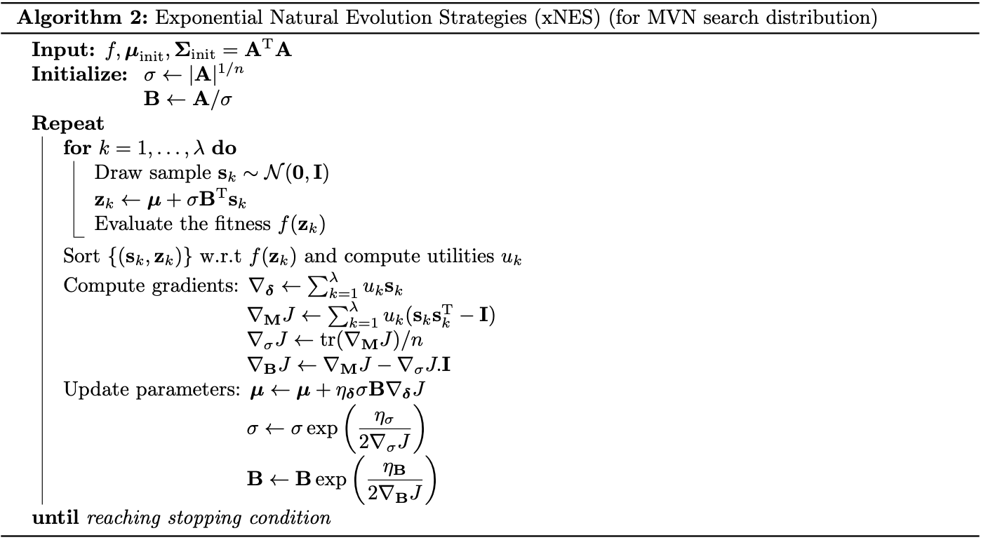
Differentiating \eqref{eq:xnes.1} w.r.t $r^2$ then gives us \begin{equation} q_\boldsymbol{\tau}’(r^2)=\frac{\partial}{\partial(r^2)}\frac{1}{(2\pi)^{n/2}}\exp\left(-\frac{1}{2}r^2\right)=-\frac{1}{2}\frac{1}{(2\pi)^{n/2}}\exp\left(-\frac{1}{2}r^2\right)=-\frac{1}{2}q_\boldsymbol{\tau}(r^2), \end{equation} which by \eqref{eq:ec.2} and \eqref{eq:ec.3} implies that \begin{equation} \mathbf{g}_\boldsymbol{\delta}=-2\frac{q_\boldsymbol{\tau}’(\Vert\mathbf{s}\Vert^2)}{q_\boldsymbol{\tau}(\Vert\mathbf{s}\Vert^2)}\mathbf{s}=\mathbf{s} \end{equation} and \begin{equation} \mathbf{g}_\mathbf{M}=-\frac{1}{2}\mathbf{I}-\frac{q_\boldsymbol{\tau}’(\Vert\mathbf{s}\Vert^2)}{q_\boldsymbol{\tau}(\Vert\mathbf{s}\Vert^2)}\mathbf{s}\mathbf{s}^\text{T}=\frac{1}{2}(\mathbf{s}\mathbf{s}^\text{T}-\mathbf{I}) \end{equation} Hence, the natural gradient is then given as \begin{align} \nabla_\boldsymbol{\delta}J&=\sum_{k=1}^{\lambda}f(\mathbf{z}_k)\mathbf{s}_k \\ \nabla_\mathbf{M}J&=\sum_{k=1}^{\lambda}f(\mathbf{z}_k)(\mathbf{s}_k\mathbf{s}_k^\text{T}-\mathbf{I}), \end{align} which can be improved with fitness shaping using the update formula \eqref{eq:fs.1} as \begin{align} \nabla_\boldsymbol{\delta}J&=\sum_{k=1}^{\lambda}u_k\mathbf{s}_{k:\lambda}, \\ \nabla_\mathbf{M}J&=\sum_{k=1}^{\lambda}u_k(\mathbf{s}_{k:\lambda}\mathbf{s}_{k:\lambda}^\text{T}-\mathbf{I}), \end{align} where $\mathbf{s}_{k:\lambda}$ denotes the $k$-th best sample in local coordinates. The resulting algorithm is thus known as Exponential Natural Evolution Strategies, or xNES, with the corresponding pseudocode shown below.
Testing on Rastrigin function
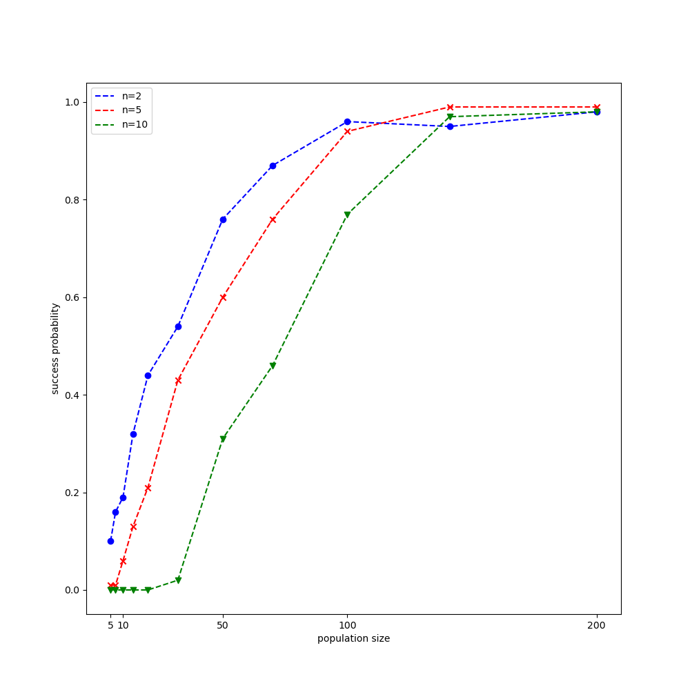
Analogy to CMA-ES, let us test NES on the Rastrigin function, which is, recall that, given by the formula \begin{equation} f(\mathbf{x})=10 n+\sum_{i=1}^{n}x_i^2-10\cos\left(2\pi x_i\right) \end{equation} $f(\mathbf{x})$ reaches its global minimum $0$ at $\mathbf{x}=\mathbf{0}$. The experimental setup we are going to use are provided in Wierstra et al. 2014. Similar to our test with CMA-ES, each function evaluation is counted as success when it reaches $f_\text{stop}=10^{-10}$.
The result after running our experiment is illustrated in the figure below.
References
[1] Daan Wierstra, Tom Schaul, Jan Peters, Jürgen Schmidhuber. Natural Evolution Strategies. IEEE World Congress on Computational Intelligence, 2008.
[2] Daan Wierstra, Tom Schaul, Tobias Glasmachers, Yi Sun, Jürgen Schmidhuber. Natural Evolution Strategies. arXiv:1106.4487, 2011.
[3] Daan Wierstra, Tom Schaul, Tobias Glasmachers, Yi Sun, Jan Peters, Jürgen Schmidhuber. Natural Evolution Strategies. Journal of Machine Learning Research 15, 2014.
[4] Jan Reinhard Peters. Machine Learning of Motor Skills for Robotics. PhD thesis, 2007.
[5] Stephen Boyd & Lieven Vandenberghe. Convex Optimization. Cambridge UP, 2004.
[6] Ha, David. A Visual Guide to Evolution Strategies. blog.otoro.net, 2017.