CMA Evolution Strategy

Notes on CMA - Evolution Strategy.

Preliminaries

The condition number of a matrix $\mathbf{A}$ is defined by \begin{equation} \kappa(\mathbf{A})\doteq\Vert\mathbf{A}\Vert\Vert\mathbf{A}^{-1}\Vert, \end{equation} where $\Vert\mathbf{A}\Vert=\sup_{\Vert\mathbf{x}\Vert=1}\Vert\mathbf{Ax}\Vert$.

For $\mathbf{A}$ that is non-singular, $\kappa(\mathbf{A})=\infty$.

For $\mathbf{A}$ which is positive definite, we thus have $\Vert\mathbf{A}\Vert=\lambda_\text{max}$ where $\lambda_\text{max}$ denotes the largest eigenvalue of $\mathbf{A}$, correspondingly $\lambda_\text{min}$ denotes the smallest eigenvalue of $\mathbf{A}$. The condition number of $\mathbf{A}$ therefore can be written as \begin{equation} \kappa(\mathbf{A})=\frac{\lambda_\text{max}}{\lambda_\text{min}}\geq 1, \end{equation} since corresponding to each eigenvalue $\lambda$ of $\mathbf{A}$, the inverse matrix $\mathbf{A}^{-1}$ takes $1/\lambda$ as its eigenvalue.

Basic equation

In the CMA-ES, a population of new search points is generated by sampling an MVN, in which at generation $t+1$, for $t=0,1,2,\ldots$ \begin{equation} \mathbf{x}_k^{(t+1)}\sim\boldsymbol{\mu}^{(t)}+\sigma^{(t)}\mathcal{N}(\mathbf{0},\boldsymbol{\Sigma}^{(t)})\sim\mathcal{N}\left(\boldsymbol{\mu}^{(t)},{\sigma^{(t)}}^2\boldsymbol{\Sigma}^{(t)}\right),\hspace{1cm}k=1,\ldots,\lambda\label{eq:be.1} \end{equation} where

• $\mathbf{x}_k^{(t+1)}\in\mathbb{R}^n$: the $k$-th sample at generation $t+1$.
• $\boldsymbol{\mu}^{(t)}\in\mathbb{R}^n$: mean of the search distribution at generation $t$.
• $\sigma^{(t)}\in\mathbb{R}$: step-size at generation $t$.
• $\boldsymbol{\Sigma}^{(t)}$: covariance matrix at generation $t$.
• ${\sigma^{(t)}}^2\boldsymbol{\Sigma}^{(t)}$: covariance matrix of the search distribution at generation $t$.
• $\lambda\geq 2$: sample size.

Updating the mean

The mean $\boldsymbol{\mu}^{(t+1)}$ of the search distribution is defined as the weighted average of $\gamma$ selected points from the sample $\mathbf{x}_1^{(t+1)},\ldots,\mathbf{x}_\lambda^{(t+1)}$: \begin{equation} \boldsymbol{\mu}^{(t+1)}=\sum_{i=1}^{\gamma}w_i\mathbf{x}_{i:\lambda}^{(t+1)},\label{eq:um.1} \end{equation} where

• $\sum_{i=1}^{\gamma}w_i=1$ with $w_1\geq w_2\geq\ldots\geq w_{\gamma}>0$.
• $\gamma\leq\lambda$: number of selected points.
• $\mathbf{x}_{i:\lambda}^{(t+1)}$: $i$-th best sample out of $\mathbf{x}_1^{(t+1)},\ldots,\mathbf{x}_\lambda^{(t+1)}$ from \eqref{eq:be.1}, i.e. with $f$ is the objective function to be minimized, we have \begin{equation} f(\mathbf{x}_{1:\lambda}^{(t+1)})\geq f(\mathbf{x}_{2:\lambda}^{(t+1)})\geq\ldots\geq f(\mathbf{x}_{\lambda:\lambda}^{(t+1)}) \end{equation}

We can rewrite \eqref{eq:um.1} as an update rule for the mean $\boldsymbol{\mu}$ \begin{equation} \boldsymbol{\mu}^{(t+1)}=\boldsymbol{\mu}^{(t)}+\alpha_\boldsymbol{\mu}\sum_{i=1}^{\gamma}w_i\left(\mathbf{x}_{i:\lambda}^{(t+1)}-\boldsymbol{\mu}^{(t)}\right), \end{equation} where $\alpha_\boldsymbol{\mu}\leq 1$ is the learning rate, which is usually set to $1$.

When choosing the weight values $w_i$ and population size $\gamma$ for recombination, we take into account the variance effective selection mass, denoted as $\gamma_\text{eff}$, given by \begin{equation} \gamma_\text{eff}\doteq\left(\frac{\Vert\mathbf{w}\Vert_1}{\Vert\mathbf{w}\Vert_2}\right)=\frac{\Vert\mathbf{w}\Vert_1^2}{\Vert\mathbf{w}\Vert_2^2}=\frac{1}{\sum_{i=1}^{\gamma}w_i^2} \end{equation} where $\mathbf{w}$ is defined as the weight vector \begin{equation} \mathbf{w}=(w_1,\ldots,w_\gamma)^\text{T} \end{equation}

Adapting the covariance matrix

The covariance matrix can be estimated from scratch using the population of the current generation or can be estimated with covariance matrix from previous generations.

Estimating from scratch

Rather than using the empirical covariance matrix as an estimator for $\boldsymbol{\Sigma}^{(t)}$, in the CMA-ES, we consider the following estimation \begin{equation} \boldsymbol{\Sigma}_\lambda^{(t+1)}=\frac{1}{\lambda{\sigma^{(t)}}^2}\sum_{i=1}^{\lambda}\left(\mathbf{x}_i^{(t+1)}-\boldsymbol{\mu}^{(t)}\right)\left(\mathbf{x}_i^{(t+1)}-\boldsymbol{\mu}^{(t)}\right)^\text{T}\label{eq:es.1} \end{equation} Notice that in the above estimation \eqref{eq:es.1}, we have used all of the $\lambda$ samples. We thus can estimate a better covariance matrix by select some of the best individual out of $\lambda$ samples, which is analogous to how we update the mean $\boldsymbol{\mu}$.

In particular, we instead consider the estimation \begin{equation} \boldsymbol{\Sigma}_{\gamma}^{(t+1)}=\frac{1}{{\sigma^{(t)}}^2}\sum_{i=1}^{\gamma}w_i\left(\mathbf{x}_{i:\lambda}^{(t+1)}-\boldsymbol{\mu}^{(t)}\right)\left(\mathbf{x}_{i:\lambda}^{(t+1)}-\boldsymbol{\mu}^{(t)}\right)^\text{T},\label{eq:es.2} \end{equation} where $\gamma\leq\lambda$ is the number of selected points; the weights $w_i$ and selected points $\mathbf{x}_{i:\lambda}^{(t+1)}$ are defined as given in the update for $\boldsymbol{\mu}$.

Rank-$\gamma$ update

In order to ensure that \eqref{eq:es.2} is a reliable estimator, the selected population must be large enough. However, to get a fast search, the population size $\lambda$ must be small, which lets the selected sample size consequently small also. Thus, we can not get a reliable estimator for a good covariance matrix from \eqref{eq:es.2}. However, we can use the history as a helping hand.

In particular, if we have experienced a sufficient number of generations, the mean of the $\boldsymbol{\Sigma}_\gamma$ from all previous generations \begin{equation} \boldsymbol{\Sigma}^{(t+1)}=\frac{1}{t+1}\sum_{i=0}^{t}\boldsymbol{\Sigma}_\gamma^{(i+1)}\label{eq:rlmu.1} \end{equation} would be a reliable estimator.

In addition, it is reasonable that the recent generations will have more affection to the current generation than the distant ones. Hence, rather than assigning estimated covariance matrices $\boldsymbol{\Sigma}_\gamma$ from preceding generations the same weight as in \eqref{eq:rlmu.1}, it would be a better choice to give the more recent generations the higher weight.

Specifically, starting with an initial $\boldsymbol{\Sigma}^{(0)}=\mathbf{I}$, we consider the update, called rank-$\gamma$ update, for the covariance matrix at generation $t+1$ using exponential smoothing¹ as \begin{align} \boldsymbol{\Sigma}^{(t+1)}&=(1-\alpha_\gamma)\boldsymbol{\Sigma}^{(t)}+\alpha_\gamma\boldsymbol{\Sigma}_\gamma^{(t+1)} \\ &=(1-\alpha_\gamma)\boldsymbol{\Sigma}^{(t)}+\alpha_\gamma\frac{1}{{\sigma^{(t)}}^2}\sum_{i=1}^{\gamma}w_i\left(\mathbf{x}_{i:\lambda}^{(t+1)}-\boldsymbol{\mu}^{(t)}\right)\left(\mathbf{x}_{i:\lambda}^{(t+1)}-\boldsymbol{\mu}^{(t)}\right)^\text{T} \\ &=(1-\alpha_\gamma)\boldsymbol{\Sigma}^{(t)}+\alpha_\gamma\sum_{i=1}^{\gamma}w_i\mathbf{y}_{i:\lambda}^{(t+1)}{\mathbf{y}_{i:\lambda}^{(t+1)}}^\text{T},\label{eq:rlmu.2} \end{align} where

• $\alpha_\gamma\leq 1$: learning rate.
• $w_1,\ldots,w_\gamma$ and $\mathbf{x}_{1:\lambda}^{(t+1)},\ldots,\mathbf{x}_{\lambda:\lambda}^{(g+1)}$ are defined as usual.
• $\mathbf{y}_{i:\lambda}^{(t+1)}=(\mathbf{x}_{i:\lambda}^{(t+1)}-\boldsymbol{\mu}^{(t)})/\sigma^{(t)}$.

The update \eqref{eq:rlmu.2} can be generalized to $\lambda$ weights values which neither necessarily sum to $1$, nor be non-negative anymore, as \begin{align} \boldsymbol{\Sigma}^{(t+1)}&=\left(1-\alpha_\gamma\sum_{i=1}^{\lambda}w_i\right)\boldsymbol{\Sigma}^{(t)}+\alpha_\gamma\sum_{i=1}^{\lambda}w_i\mathbf{y}_{i:\lambda}^{(t+1)}{\mathbf{y}_{i:\lambda}^{(t+1)}}^\text{T}\label{eq:rlmu.3} \\ &={\boldsymbol{\Sigma}^{(t)}}^{1/2}\left[\mathbf{I}+\alpha_\gamma\sum_{i=1}^{\lambda}w_i\left(\mathbf{z}_{i:\lambda}^{(t+1)}{\mathbf{z}_{i:\lambda}^{(t+1)}}^\text{T}-\mathbf{I}\right)\right]{\boldsymbol{\Sigma}^{(t)}}^{1/2}, \end{align} where

• $w_1\geq\ldots\geq w_\gamma>0\geq w_{\gamma+1}\geq\ldots\geq w_\lambda\in\mathbb{R}$, and usually $\sum_{i=1}^{\gamma}w_i=1$ and $\sum_{i=1}^{\lambda}w_i\approx 0$.
• $\mathbf{z}_{i:\lambda}^{(t+1)}={\boldsymbol{\Sigma}^{(t)}}^{1/2}\mathbf{y}_{i:\lambda}^{(t+1)}$ is the mutation vector.

Rank-one-update

We first consider a method that produces an $n$-dimensional normal distribution with zero mean. Specifically, let $\mathbf{y}_1,\ldots,\mathbf{y}_{t_0}\in\mathbb{R}^n$, for $t_0\geq n$ be vectors span $\mathbb{R}^n$. We thus have that \begin{align} \mathcal{N}(0,1)\mathbf{y}_1+\ldots+\mathcal{N}(0,1)\mathbf{y}_{t_0}&\sim\mathcal{N}(\mathbf{0},\mathbf{y}_1\mathbf{y}_1^\text{T})+\ldots+\mathcal{N}(\mathbf{0},\mathbf{y}_{t_0}\mathbf{y}_{t_0}^\text{T}) \\ &\sim\mathcal{N}\left(\mathbf{0},\sum_{i=1}^{t_0}\mathbf{y}_i\mathbf{y}_i^\text{T}\right) \end{align} The covariance matrix $\mathbf{y}_i\mathbf{y}_i^\text{T}$ has rank one, with only one eigenvalue $\Vert\mathbf{y}_i\Vert^2$ and a corresponding eigenvector within the form $\alpha\mathbf{y}_i$ for $\alpha\in\mathbb{R}$. Using the above equation, we can generate any MVN distribution.

Consider the update \eqref{eq:rlmu.3} with $\gamma=1$ and let $\mathbf{y}_{t+1}=\left(\mathbf{x}_{1:\lambda}^{(t+1)}-\boldsymbol{\mu}^{(t)}\right)/\sigma^{(t)}$, the rank-one update for the covariance matrix $\boldsymbol{\Sigma}^{(t+1)}$ is given by \begin{equation} \boldsymbol{\Sigma}^{t+1}=(1-\alpha_1)\boldsymbol{\Sigma}^{(t)}+\alpha_1\mathbf{y}_{t+1}\mathbf{y}_{t+1}^\text{T} \end{equation} The latter summand in the RHS has rank one and adds the maximum likelihood term for $\mathbf{y}_{t+1}$ into the covariance matrix $\boldsymbol{\Sigma}^{(t)}$, which makes the probability of generating $\mathbf{y}_{t+1}$ in the generation $t+1$ increase.

We continue by noticing that to update the covariance matrix $\boldsymbol{\Sigma}^{(t+1)}$, in \eqref{eq:rlmu.3}, we have used the selected steps \begin{equation} \mathbf{y}_{i:\lambda}^{(g+1)}=\frac{\mathbf{x}_{i:\lambda}^{(g+1)}-\boldsymbol{\mu}^{(g)}}{\sigma^{(g)}} \end{equation} However, since \begin{equation} \mathbf{y}_{i:\lambda}^{(g+1)}{\mathbf{y}_{i:\lambda}^{(g+1)}}^\text{T}=-\mathbf{y}_{i:\lambda}^{(g+1)}\left(-\mathbf{y}_{i:\lambda}^{(g+1)}\right)^\text{T}, \end{equation} which means the sign information is lost when computing the covariance matrix. To track the sign information to the update rule of $\boldsymbol{\Sigma}^{(t+1)}$, we use evolution path, which defined as a sequence of successive steps over number of generations.

In particular, analogy to \eqref{eq:rlmu.3}, we use exponential smoothing to establish the evolution path, $\mathbf{p}_c\in\mathbb{R}^n$, which starting with an initial value $\mathbf{p}_c^{(0)}=\mathbf{0}$ and being updated with \begin{align} \mathbf{p}_c^{(t+1)}&=(1-\alpha_c)\mathbf{p}_c^{(t)}+\sqrt{(1-(1-\alpha_c)^2)\mu_\text{eff}}\sum_{i=1}^{\gamma}w_i\mathbf{y}_{i:\lambda}^{(t+1)} \\ &=(1-\alpha_c)\mathbf{p}_c^{(t)}+\sqrt{\alpha_c(2-\alpha_c)\gamma_\text{eff}}\sum_{i=1}^{\gamma}\frac{w_i\left(\mathbf{x}_{i:\lambda}^{(t+1)}-\boldsymbol{\mu}^{(t)}\right)}{\sigma^{(t)}} \\ &=(1-\alpha_c)\mathbf{p}_c^{(t)}+\sqrt{\alpha_c(2-\alpha_c)\gamma_\text{eff}}\frac{1}{\sigma^{(t)}}\left[\left(\sum_{i=1}^{\gamma}w_i\mathbf{x}_{i:\lambda}^{(t+1)}\right)-\boldsymbol{\mu}^{(t)}\sum_{i=1}^{\gamma}w_i\right] \\ &=(1-\alpha_c)\mathbf{p}_c^{(t)}+\sqrt{\alpha_c(2-\alpha_c)\gamma_\text{eff}}\frac{\boldsymbol{\mu}^{(t+1)}-\boldsymbol{\mu}^{(t)}}{\sigma^{(t)}}, \end{align} where

• $\mathbf{p}_c^{(t)}\in\mathbb{R}^n$ is the evolution path at generation $t$.
• $\alpha_c\leq 1$ is the learning rate.
• $\sqrt{\alpha_c(2-\alpha_c)\gamma_\text{eff}}$ is a normalization factor for $\mathbf{p}_c^{(t+1)}$ such that \begin{equation} \mathbf{p}_c^{(t+1)}\sim\mathcal{N}(\mathbf{0},\boldsymbol{\Sigma}), \end{equation} since by $\mathbf{y}_{i:\lambda}^{(t+1)}=(\mathbf{x}_{i:\lambda}^{(t+1)}-\boldsymbol{\mu}^{(t)})/\sigma^{(t)}$ we have that \begin{equation} \mathbf{p}_c^{(t)}\sim\mathbf{y}_{i:\lambda}^{(t+1)}\sim\mathcal{N}(\mathbf{0},\boldsymbol{\Sigma}),\hspace{1cm}\forall i=1,\ldots,\gamma \end{equation} which by $\gamma_\text{eff}=\left(\sum_{i=1}^{\gamma}w_i^2\right)^{-1}$ implies that \begin{equation} \sum_{i=1}^{\gamma}w_i\mathbf{y}_{i:\lambda}^{(t+1)}\sim\frac{1}{\sqrt{\gamma_\text{eff}}}\mathcal{N}(\mathbf{0},\boldsymbol{\Sigma}) \end{equation}

The rank-one update for the covariance matrix $\boldsymbol{\Sigma}^{(t)}$ via the evolution path $\mathbf{p}_c^{(t+1)}$ then given as \begin{equation} \boldsymbol{\Sigma}^{(t+1)}=(1-\alpha_1)\boldsymbol{\Sigma}^{(t)}+\alpha_1\mathbf{p}_c^{(t+1)}{\mathbf{p}_c^{(t+1)}}^\text{T},\label{eq:rou.1} \end{equation} An empirical validated choice for the learning rate $\alpha_1$ is $\alpha_1\approx 2/n^2$.

Final update

Combining rank-$\gamma$ update \eqref{eq:rlmu.3} and rank-one update \eqref{eq:rou.1} together, we obtain the final update for the covariance matrix $\boldsymbol{\Sigma}^{(t+1)}$ as \begin{equation} \boldsymbol{\Sigma}^{(t+1)}=\left(1-\alpha_1-\alpha_\gamma\sum_{i=1}^{\lambda}w_i\right)\boldsymbol{\Sigma}^{(t)}+\alpha_1\mathbf{p}_c^{(t+1)}{\mathbf{p}_c^{(t+1)}}^\text{T}+\alpha_\gamma\sum_{i=1}^{\lambda}w_i\mathbf{y}_{i:\lambda}^{(t+1)}{\mathbf{y}_{i:\lambda}^{(t+1)}}^\text{T}, \end{equation} where

• $\alpha_1\approx 2/n^2$.
• $\alpha_\gamma\approx\min(\gamma_\text{eff}/n^2,1-\alpha_1)$.
• $\mathbf{y}_{i:\lambda}^{(t+1)}=\left(\mathbf{x}_{i:\lambda}^{(t+1)}-\boldsymbol{\mu}^{(t)}\right)/\sigma^{(t)}$.
• $\sum_{i=1}^{\lambda}w_i\approx-\alpha_1/\alpha_\gamma$.

Controlling the step-size

To control the step-size $\sigma^{(t)}$, similar to how we cumulatively update the covariance matrix by rank-one covariance matrices, we also use an evolution path, which is defined as sum of successive steps $\boldsymbol{\mu}^{(t+1)}-\boldsymbol{\mu}^{(t)}$.

However, in this step-size adaption, we utilize a conjugate evolution path $\mathbf{p}_\sigma$, which begins with an initial value $\mathbf{p}_\sigma^{(0)}=\mathbf{0}$ and is repeatedly updated by \begin{align} \mathbf{p}_\sigma^{(t+1)}&=(1-\alpha_\sigma)\mathbf{p}_\sigma^{(t)}+\sqrt{(1-(1-\alpha_\sigma)^2)\gamma_\text{eff}}{\boldsymbol{\Sigma}^{(t)}}^{-1/2}\sum_{i=1}^{\gamma}w_i\mathbf{y}_{i:\lambda}^{(t+1)} \\ &=1-\alpha_\sigma)\mathbf{p}_\sigma^{(t)}+\sqrt{\alpha_\sigma(2-\alpha_\sigma)\gamma_\text{eff}}{\boldsymbol{\Sigma}^{(t)}}^{-1/2}\sum_{i=1}^{\gamma}w_i\frac{\mathbf{x}_{i:\lambda}^{(t+1)}-\boldsymbol{\mu}^{(t)}}{\sigma^{(t)}} \\ &=1-\alpha_\sigma)\mathbf{p}_\sigma^{(t)}+\sqrt{\alpha_\sigma(2-\alpha_\sigma)\gamma_\text{eff}}{\boldsymbol{\Sigma}^{(t)}}^{-1/2}\frac{1}{\sigma^{(t)}}\left[\left(\sum_{i=1}^{\gamma}w_i\mathbf{x}_{i:\lambda}^{(t+1)}\right)-\boldsymbol{\mu}^{(t)}\sum_{i=1}^{\gamma}w_i\right] \\ &=1-\alpha_\sigma)\mathbf{p}_\sigma^{(t)}+\sqrt{\alpha_\sigma(2-\alpha_\sigma)\gamma_\text{eff}}{\boldsymbol{\Sigma}^{(t)}}^{-1/2}\frac{\boldsymbol{\mu}^{(t+1)}-\boldsymbol{\mu}^{(t)}}{\sigma^{(t)}}, \end{align} where

• $\mathbf{p}_\sigma^{(t)}\in\mathbb{R}^n$ is the conjugate evolution path at generation $t$.
• $\alpha_\sigma<1$ is the learning rate.
• $\sqrt{\alpha_c(2-\alpha_c)\gamma_\text{eff}}$ is a normalization factor for $\mathbf{p}_\sigma^{(t+1)}$, which analogously to the covariance matrix adaption, lets \begin{equation} \mathbf{p}_\sigma^{(t+1)}\sim\mathcal{N}(\mathbf{0},\mathbf{I}) \end{equation}
• The covariance matrix ${\boldsymbol{\Sigma}^{(t)}}^{-1/2}$ is defined as \begin{equation} {\boldsymbol{\Sigma}^{(t)}}^{-1/2}\doteq\mathbf{Q}^{(t)}{\boldsymbol{\Lambda}^{(t)}}^{-1/2}{\mathbf{Q}^{(t)}}^\text{T},\label{eq:cs.1} \end{equation} where \begin{equation} \hspace{-0.8cm}\boldsymbol{\Sigma}^{(t)}=\mathbf{Q}^{(t)}\boldsymbol{\Lambda}^{(t)}{\mathbf{Q}^{(t)}}^\text{T}=\left[\begin{matrix}\vert&&\vert \\ \mathbf{q}_1^{(t)}&\ldots&\mathbf{q}_n^{(t)} \\ \vert&&\vert\end{matrix}\right]\left[\begin{matrix}\lambda_1^{(t)}&& \\ &\ddots& \\ && \lambda_n^{(t)}\end{matrix}\right]\left[\begin{matrix}\vert&&\vert \\ \mathbf{q}_1^{(t)}&\ldots&\mathbf{q}_n^{(t)} \\ \vert&&\vert\end{matrix}\right]^\text{T} \end{equation} is an eigendecomposition of the positive definite covariance matrix $\boldsymbol{\Sigma}^{(t)}$, where $\mathbf{Q}^{(t)}\in\mathbb{R}^{n\times n}$ is an orthonormal matrix whose columns are unit eigenvectors $\mathbf{q}_i^{(t)}$ of $\boldsymbol{\Sigma}^{(t)}$ and $\boldsymbol{\Lambda}^{(t)}\in\mathbb{R}^{n\times n}$ is a diagonal matrix whose diagonal entries are eigenvalues $\lambda_i^{(t)}$ of $\boldsymbol{\Sigma}^{(t)}$.
  Moreover, for each eigenvalue, eigenvector pair $(\lambda_i^{(t)},\mathbf{q}_i^{(t)})$ of $\boldsymbol{\Sigma}^{(t)}$ we have \begin{equation} \lambda_i^{(t)}{\boldsymbol{\Sigma}^{(t)}}^{-1}\mathbf{q}_i^{(t)}={\boldsymbol{\Sigma}^{(t)}}^{-1}\boldsymbol{\Sigma}^{(t)}\mathbf{q}_i^{(t)}=\mathbf{q}_i^{(t)}, \end{equation} or \begin{equation} {\boldsymbol{\Sigma}^{(t)}}^{-1}\mathbf{q}_i^{(t)}=\frac{1}{\lambda_i^{(t)}}\mathbf{q}_i^{(t)}, \end{equation} or in other words, $(1/\lambda_i^{(t)},\mathbf{q}_i^{(t)})$ is an eigenvalue, eigenvector pair of ${\boldsymbol{\Sigma}^{(t)}}^{-1}$. Therefore, the inverse of $\boldsymbol{\Sigma}^{(t)}$, which is also positive definite can be written by \begin{equation} {\boldsymbol{\Sigma}^{(t)}}^{-1}=\mathbf{Q}^{(t)}\left[\begin{matrix}1/\lambda_1^{(t)}&& \\ &\ddots& \\ && 1/\lambda_n^{(t)}\end{matrix}\right]{\mathbf{Q}^{(t)}}^\text{T}=\mathbf{Q}^{(t)}{\boldsymbol{\Lambda}^{(t)}}^{-1}{\mathbf{Q}^{(t)}}^\text{T}, \end{equation} which allows us to obtain the representation \eqref{eq:cs.1} of ${\boldsymbol{\Sigma}^{(t)}}^{-1/2}$.

The transformation ${\boldsymbol{\Sigma}^{(t)}}^{-1/2}=\mathbf{Q}^{(t)}{\boldsymbol{\Lambda}^{(t)}}^{-1/2}{\mathbf{Q}^{(t)}}^\text{T}$ re-scales length of the step $\boldsymbol{\mu}^{(t+1)}-\boldsymbol{\mu}^{(t)}$ without changing its direction. In more specific:

• ${\mathbf{Q}^{(t)}}^\text{T}$ transform the original space into the coordinate space with columns of $\mathbf{Q}^{(t)}$, which is also the eigenvectors of $\boldsymbol{\Sigma}^{(t)}$ or the principle axes of $\mathcal{N}(\mathbf{0},\boldsymbol{\Sigma}^{(t)})$, as its principle axes.
• ${\boldsymbol{\Lambda}^{(t)}}^{-1/2}$ re-scales the principle axes to have the same length.
• $\mathbf{Q}^{(t)}$ transforms the coordinate system back to the original space.

It means that this transformation makes the expected length of $\mathbf{p}_\sigma^{(t+1)}$ independent of its direction.

We then update $\sigma^{(t)}$ by according to the ratio of its length with its expected length $\Vert\mathbf{p}_\sigma^{(t+1)}\Vert/\mathbb{E}\Vert\mathcal{N}(\mathbf{0},\mathbf{I})\Vert$, given by \begin{equation} \log\sigma^{(t+1)}=\log\sigma^{(t)}+\frac{\alpha_\sigma}{d_\sigma}\left(\frac{\Vert\mathbf{p}_\sigma^{(t+1)}\Vert}{\mathbb{E}\Vert\mathcal{N}(\mathbf{0},\mathbf{I})\Vert}-1\right), \end{equation} where $d_\sigma\approx 1$ is the damping parameter, which controls the update size. Therefore, since $\sigma^{(t)}>0$, we have the update rule for $\sigma^{(t)}$ is given by \begin{equation} \sigma^{(t+1)}=\sigma^{(t)}\exp\left(\frac{\alpha_\sigma}{d_\sigma}\left(\frac{\Vert\mathbf{p}_\sigma^{(t+1)}\Vert}{\mathbb{E}\Vert\mathcal{N}(\mathbf{0},\mathbf{I})\Vert}-1\right)\right) \end{equation}

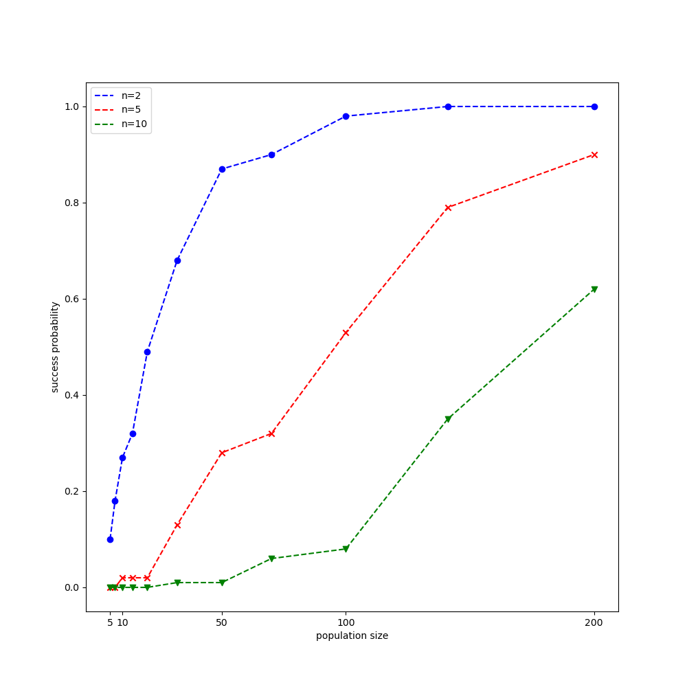
Testing on Rastrigin function

Let us give the CMA-ES algorithm a try on the Rastrigin function, $f:\mathbb{R}^n\to\mathbb{R}$, which is given by \begin{equation} f(\mathbf{x})=10 n+\sum_{i=1}^{n}x_i^2-10\cos\left(2\pi x_i\right) \end{equation} The global minimum of $f(\mathbf{x})$ is $0$ at $\mathbf{x}=\mathbf{0}$. We will be using the experimental settings given in this paper proposed by CMA-ES’s original author. Each time we end up with a result less than $f_\text{stop}=10^{-10}$, we count it a success run.

The result obtained is illustrated in the following figure.

References

[1] Nikolaus Hansen. The CMA Evolution Strategy: A Tutorial. arXiv:1604.00772, 2016.

[2] Nikolaus Hansen, Youhei Akimoto & Petr Baudis. CMA-ES/pycma on Github. Zenodo, DOI:10.5281/zenodo.2559634, February 2019.

[3] Nikolaus Hansen, Stefan Kern. Evaluating the CMA Evolution Strategy on Multimodal Test Functions. Parallel Problem Solving from Nature - PPSN VIII. PPSN 2004.

[4] Ha, David. A Visual Guide to Evolution Strategies. blog.otoro.net, 2017.

Footnotes